Page 111 - Fair, Geyer, and Okun's Water and wastewater engineering : water supply and wastewater removal

JWCL344_ch03_061-117.qxd 8/17/10 7:48 PM Page 74

74 Chapter 3 Water Sources: Groundwater
and outside the integral. Theis (1963) devised a graphical method of superposition to ob-
tain a solution of the equation for T and S.
If the discharge Q is known, the formation constants of an aquifer can be obtained as
follows:
2
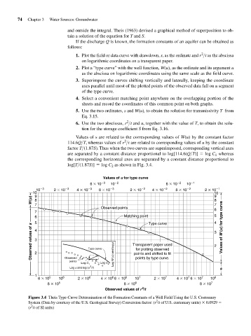
1. Plot the field or data curve with drawdown, s, as the ordinate and r >t as the abscissa
on logarithmic coordinates on a transparent paper.
2. Plot a “type curve” with the well function, W(u), as the ordinate and its argument u
as the abscissa on logarithmic coordinates using the same scale as the field curve.
3. Superimpose the curves shifting vertically and laterally, keeping the coordinate
axes parallel until most of the plotted points of the observed data fall on a segment
of the type curve.
4. Select a convenient matching point anywhere on the overlapping portion of the
sheets and record the coordinates of this common point on both graphs.
5. Use the two ordinates, s and W(u), to obtain the solution for transmissivity T from
Eq. 3.15.
2
6. Use the two abscissas, r >t and u, together with the value of T, to obtain the solu-
tion for the storage coefficient S from Eq. 3.16.
Values of s are related to the corresponding values of W(u) by the constant factor
2
114.6Q>T, whereas values of r >t are related to corresponding values of u by the constant
factor T>(1.87S) . Thus when the two curves are superimposed, corresponding vertical axes
are separated by a constant distance proportional to log[114.6(Q>T)] = log C 1 whereas
the corresponding horizontal axes are separated by a constant distance proportional to
log[T>(1.87S)] = log C 2 as shown in Fig. 3.4.

Values of u for type curve
6 10 3 10 2 6 10 2 10 1
10 3 2 10 3 4 10 3 8 10 3 2 10 2 4 10 2 8 10 2 2 10 1
10 9 10
9
W(u) 8 8
7
Observed points 7
6
7
6 Matching point 5
5 4 Type curve 4 Values of W (u) for type curve
Observed values of s 3 Type curve Transparent paper used 3

2
for plotting observed
2
points by type curve.
Observed
points Log W (u) and log p points and shifted to fit
Log C 1 Log C 2
2
Log u and log (x /t) s
1
7
6
6 10 5 10 6 2 10 6 4 10 6 10 6 10 7 2 10 7 4 10 6 10 7 10 8
8 10 5 8 10 6 8 10 7
2
Observed values of r /t
Figure 3.4 Theis Type-Curve Determination of the Formation Constants of a Well Field Using the U.S. Customary
2
System (Data by courtesy of the U.S. Geological Survey) Conversion factor: (r /t of U.S. customary units) 0.0929
2
(r /t of SI units)