Page 122 - Fair, Geyer, and Okun's Water and wastewater engineering : water supply and wastewater removal

JWCL344_ch03_061-117.qxd 8/17/10 7:48 PM Page 84

84 Chapter 3 Water Sources: Groundwater

EXAMPLE 3.4 DETERMINATION OF THE PROFILE OF A CONE OF DEPRESSION
Determine the profile of a quasi-steady-state cone of depression for a proposed 24-in. (61-cm) well
pumping continuously at (a) 150 gpm, (b) 200 gpm, and (c) 250 gpm in an elastic artesian aquifer
4
having a transmissivity of 10,000 gpd/ft and a storage coefficient of 6 10 . Assume that the dis-
charge and recharge conditions are such that the drawdowns will be stabilized after 180 days.
Solution:
The distance at which drawdown is approaching zero, that is, the radius of cone of depression, can
be obtained from Eq. 3.24:
2
r 0 0.3 Tt>S 0.3 Dt where D is the diffusivity of the aquifer T>S
4
4
0.3(1 l0 )180>(6 l0 ) 9 l0 8
4
4
r 0 (0.3Dt) 0.5 3 l0 ft (0.914 10 m)
This is independent of Q and depends only on the diffusivity of the aquifer. The change in draw-
down per log cycle from Eq. 3.23 is:
s 528 Q>T
4
For 150 gpm: s 1 528 150>1 10 7.9 ft (2.4 m)
For 200 gpm: s 2 10.6 ft (3.23 m)
For 250 gpm: s 3 13.2 ft (4.02 m)
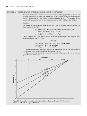
Using the value of r 30,000 ft (9,144 m) as the starting point, straight lines having slopes of
7.9, 10.6, and 13.2 ft (2.4 m, 3.2 m, 4.0 m) are drawn in Fig. 3.8.
The contours of the piezometric surface can be drawn by subtracting the drawdowns at several
points from the initial values.

Distance in ft
1 10 100 1,000 10,000
0

10
Q 150 gpm
Q 200 gpm
20 Q 250 gpm
Drawdown, ft 30

40

50

60
Figure 3.8 Distance-Drawdown Curves for Various Rates of Pumping (Example 3.4). Conversion
3
factors: 1 ft 0.3048 m; 1 gpm 5.45 m /d