Page 119 - Fair, Geyer, and Okun's Water and wastewater engineering : water supply and wastewater removal

JWCL344_ch03_061-117.qxd 8/17/10 7:48 PM Page 82

82 Chapter 3 Water Sources: Groundwater

10 2

Nonequilibrium
10 type curve 0.01 0.005 0.001
0.03 0.015
0.05
0.075
0.1
0.15
0.2
0.3
0.4
W (u, r/B) 10 1.0 0.8 0.7 0.6 s 114.6 Q W(u, r/B)
0.5
T
1.5
2
u 1.87 r S
2.0 Tt
r r
r/B 2.5
0.1 B T
(k´/b´ )
0.01
10 1 1.0 10 10 2 10 3 10 4 10 5 10 6 10 7
1

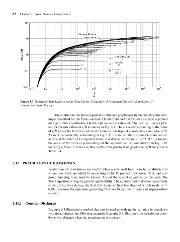
Figure 3.7 Nonsteady-State Leaky Artesian-Type Curves. Using the U.S. Customary System (After Walton of
Illinois State Water Survey)

The solution to the above equation is obtained graphically by the match-point tech-
nique described for the Theis solution. On the field curve drawdown vs. time is plotted
on logarithmic coordinates. On the type curve the values of W(u, r>B) vs. 1>u are plot-
ted for various values of r>B as shown in Fig. 3.7. The curve corresponding to the value
of r>B giving the best fit is selected. From the match-point coordinates s and W(u, r>B),
T can be calculated by substituting in Eq. 3.31. From the other two match-point coordi-
nates and the value of T computed above, S is determined from Eq. 3.32. If b is known,
the value of the vertical permeability of the aquitard can be computed from Eq. 3.30,
knowing r>B and T. Values of W(u, r>B) for the practical range of u and r>B are given in
Table 3.4.

3.11 PREDICTION OF DRAWDOWN
Predictions of drawdowns are useful when a new well field is to be established or
where new wells are added to an existing field. To predict drawdowns, T, S, and pro-
posed pumping rates must be known. Any of the several equations can be used. The
Theis equation is of quite general applicability. The approximation does not accurately
show drawdowns during the first few hours or first few days of withdrawals (u
0.01). Because the equations governing flow are linear, the principle of superposition
is valid.

3.11.1 Constant Discharge
Example 3.3 illustrated a method that can be used to evaluate the variation in drawdown
with time, whereas the following example, Example 3.4, illustrates the variation in draw-
down with distance when the pumping rate is constant.