Page 146 - Finite Element Analysis with ANSYS Workbench

8.1 Buckling 137

2
P cr ( 1mode )   2 EI L
This critical bucking load corresponds to the first mode shape.
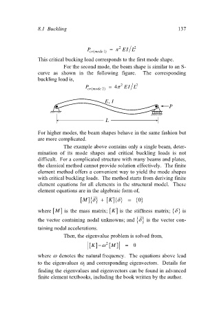
For the second mode, the beam shape is similar to an S-
curve as shown in the following figure. The corresponding
buckling load is,
2
P cr ( 2mode )  4 2 EI L

E, I
P

L

For higher modes, the beam shapes behave in the same fashion but
are more complicated.
The example above contains only a single beam, deter-

mination of its mode shapes and critical buckling loads is not
difficult. For a complicated structure with many beams and plates,
the classical method cannot provide solution effectively. The finite
element method offers a convenient way to yield the mode shapes
with critical buckling loads. The method starts from deriving finite
element equations for all elements in the structural model. These
element equations are in the algebraic form of,
    M       K    0


where   is the mass matrix;   is the stiffness matrix;   is
K
M

the vector containing nodal unknowns; and    is the vector con-
taining nodal accelerations.
Then, the eigenvalue problem is solved from,
  K 2    0
M
where  denotes the natural frequency. The equations above lead
to the eigenvalues  and corresponding eigenvectors. Details for
i
finding the eigenvalues and eigenvectors can be found in advanced
finite element textbooks, including the book written by the author.