Page 241 - Finite Element Analysis with ANSYS Workbench

232 Chapter 12 Compressible Flow Analysis

12.1 Basic Equations

12.1.1 Differential Equations
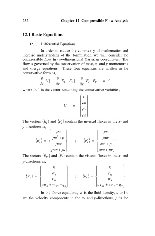
In order to reduce the complexity of mathematics and
increase understanding of the formulation, we will consider the
compressible flow in two-dimensional Cartesian coordinates. The
flow is governed by the conservation of mass, x- and y-momentums
and energy equations. These four equations are written in the
conservative form as,
     E     E F  0
F 
U
t  x  I V y  I V
where   is the vector containing the conservative variables,
U
  
  u 
    
U


  v 
   

The vectors E and   contain the inviscid fluxes in the x- and
F
I
I
y-directions as,
  u    v 
  u  p    uv 
2
F
E
       ;     2 


I
I
  uv    v  p 
   
v 
u 
  pu    pv 
The vectors  V E and   contain the viscous fluxes in the x- and
F
V
y-directions as,
 0   0 
     
 V E   x  ;     xy 
F




V
  xy    y 
u  v  q  u  v  q 
 x xy x   xy y y 
In the above equations,  is the fluid density, u and v
are the velocity components in the x- and y-directions, p is the