Page 179 - Finite Element Modeling and Simulations with ANSYS Workbench

164 Finite Element Modeling and Simulation with ANSYS Workbench

The disadvantages of using the substructuring technique are

• Increased overhead for file management
• Increased initial time for setting up the system
• Matrix condensations for dynamic problems introduce new approximations

5.4 Equation Solving
There are two types of solvers used in the FEA for solving the linear systems of algebraic
equations, mainly, the direct methods and iterative methods.

5.4.1 Direct Methods (Gauss Elimination)

• Solution time proportional to NB (with N being the dimension of the matrix and
2
B the bandwidth of the FEA systems)
• Suitable for small to medium problems (with DOFs in the 100,000 range), or slen-
der structures (small bandwidth)
• Easy to handle multiple load cases

5.4.2 Iterative Methods

• Solution time is unknown beforehand
• Reduced storage requirement
• Suitable for large problems, or bulky structures (large bandwidth, converge
faster)
• Need to solve the system again for different load cases

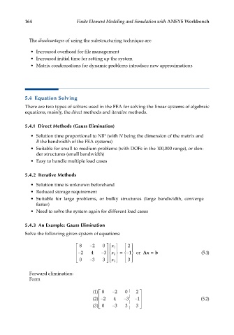
5.4.3 An Example: Gauss Elimination
Solve the following given system of equations:

 8 − 2 0 x 1   2 
 

 − 2 4 − 3  x   1  or Ax = b (5.1)
=

  2 =−

 0 − 3 3  x 3    3 
   
Forward elimination:
Form
1 
() 8 − 2 0 | 2 

() − 2 4 − 3 | − 1   (5.2)
2

3 
() 0 − 3 3 | 3 
 | 