Page 180 - Finite Element Modeling and Simulations with ANSYS Workbench

Modeling and Solution Techniques 165

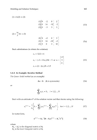
(1) + 4x(2) ⇒ (2):

() 8  − 2 0 | 2 
1

2
() 0 14 − 12 | − 2   (5.3)

() 0   − 3 3 | 3  
3
|
14
(2) + (3) ⇒ (3)
3
() 8  − 2 0 | 2 
1

() 0 14 − 12 | − 2   (5.4)
2

() 0   0 2 | 12  
3
|
Back substitutions (to obtain the solution):
x 3 = 12 2 = 6
/
 . 15


x 2 =− + 12 )/ 5 or x =  5  (5.5)
x 3 14 =
(
2
 
 6 
x 1 = ( 2 + 2 )/
x 2 8 = 115.

5.4.4 An Example: Iterative Method
The Gauss–Seidel method (as an example):
Ax = b (A is symmetric) (5.6)

or

N
∑ ax j = b i , i = , ,..., N
12
ij
j=1
Start with an estimate x of the solution vector and then iterate using the following:
(0)
 i−1 N 
1
k ( +1 ) =  b i − ∑ k ( +1 ) − ∑ k () ,  foor i = 12,,..., N (5.7)
ij
x i a x j a x j
ij
a ii  
 j=1 ji =+1 
In vector form,
()
T
k
x (k+1 ) = −1 b [ − A x (k+1 ) − A x ] (5.8)
A D L L
where
A = 〈a 〉 is the diagonal matrix of A,
D
ii
A is the lower triangular matrix of A,
L