Page 229 - Finite Element Modeling and Simulations with ANSYS Workbench

214 Finite Element Modeling and Simulation with ANSYS Workbench

6.6 Summary
In this chapter, the main aspects of the plate and shell theories and the plate and shell ele-
ments used for analyzing plate and shell structures are discussed. Plates and shells can
be regarded as the extensions of the beam elements from 1-D line elements to 2-D surface
elements. Plates are usually applied in modeling flat thin structure members, while the
shells are applied in modeling curved thin structure members. In applying the plate and
shell elements, one should keep in mind the assumptions used in the development of these
types of elements. In cases where these assumptions are no longer valid, one should turn
to general 3-D theories and solid elements. A showcase using shell elements in modeling a
vase is introduced using ANSYS Workbench.

6.7 Review of Learning Objectives

Now that you have finished this chapter you should be able to

1. Understand the assumptions used in the plate and shell theories.
2. Understand the behaviors of the plate and shell elements.
3. Know when not to use plate and shell elements in stress analysis (e.g., when plate
or shell structures have nonuniform thickness or small features).
4. Create FEA models using plate and shell elements for deformation and stress anal-
ysis using ANSYS Workbench.

PROBLEMS
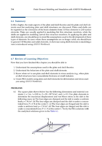
6.1 The square plate shown below has the following dimensions and material con-
stants: L = 1 m, t = 0.02 m, E = 30 × 10 N/m , and ν = 0.3. Use plate elements to
6
2
determine the maximum displacement and von Mises stress in the slab in the
following cases: (a) The four edges are clamped and the slab is under a uniform
load q = 1 N/m . (b) The four edges are clamped and the slab is under a concen-
2
trated force P = 1 N at the center C. (c) The four edges are hinged and the slab is
under a uniform load q = 1 N/m . (d) The four edges are hinged and the slab is
2
under a concentrated force P = 1 N at the center C. Verify the FEA solutions with
the analytical solutions given in the Table 6.1.

z

y
C
L

x L