Page 263 - Fluid-Structure Interactions Slender Structure and Axial Flow (Volume 1)

244 SLENDER STRUCTURES AND AXIAL FLOW

It is now presumed that there are regions in the {w, p}-plane where, for any given on,
there exist amplified oscillations or parametric resonances, and hence on the boundaries
of these regions the oscillation is purely periodic. Since a periodic solution may be repre-
sented by a Fourier series, to obtain the primary resonances, q(t) may be expressed as
q = {ak sin(ikwt) + bk cos(ikwt)}. (4.71)
k=1,3,5, ...
Substitution of equation (4.71) into (4.70) yields an infinite set of algebraic equations
which, because of the presence of sin ut, cos wt and cos2 wt terms in (4.70)
already, involves terms in sin( imwt) and cos(imot), m = k - 4, k - 2, k, k + 2, k + 4
(Paidoussis & Issid 1974). Upon expanding this equation for k = 1,3,5,. . ., and
collecting terms in cos iws, sin $in, cos iws, etc., the coefficients of which must vanish
independently, one obtains a matrix equation of the form

(4.72)
I I
bj
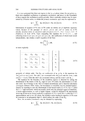
or more explicitly

..........................

I... G31 G32 G34 ..
G33

= {O}, (4.73)

G- ..
..........................

generally of infinite order. The Gjk are coefficients of ak or bk in the equations for
sin(ijwt) or cos(~jwt). The odd j are associated with sin(ijwt) and the even j with
cos[i(j - l)wt]; while the odd k are associated with ak and the even k with bk-1.
The equation for the boundary of the instability regions is obtained by setting the
determinant of the matrix of the Gjk equal to zero. Of course the determinant is of infi-
nite order, but it belongs to the class of normal determinants and is therefore absolutely
convergent (Bolotin 1964). Hence, the boundaries of instability may be obtained approx-
imately by equating to zero the determinant of the boxed matrix in (4.73); this is called
the k = 1 approximation, which necessarily yields only the principal region of instability.
A better approximation, as well as higher regions, would be obtained if the determinant
involving all the terms shown explicitly in equation (4.73) is used; this is called the k = 3
approximation; and so on. Of course, the Galerkin series leading to equation (4.70) must
be truncated at an adequately high N, which defines the order of the Gjk.
Now, the secondary resonances may be obtained by expressing

q = {ak sin(ikwt) + bk cos(ikwt)}, (4.74)
k=O. 2.4. ...