Page 363 - Fluid-Structure Interactions Slender Structure and Axial Flow (Volume 1)

PIPES CONVEYING FLUID: NONLINEAR AND CHAOTIC DYNAMICS 343

the first two of equations (5.123) and the third one are decoupled, providing immediately

4 = mot + &I + G(c).

A rescaling procedure can transform the first two equations to their usual form (Gucken-
heimer & Holmes 1983; pp. 396-411),
+
&I + r2 + k2), Z = ~(p2 CT’ + dZ2), d = &I. (5.124)

This system has been studied by Takens (1974) who found nine topologically distinct
equivalence classes. Results obtained from three different sets of parameters are presented
for comparison:
Case 1: u = 2.245 y = -46.001 B = 0.20 K = 0,

Case 2: L( = 12.598 y = 71.941 j3 = 0.18 K = 100, (5.125)
Case 3: 11 = 15.111 y = 46.88 j3 = 0.25 K = 100.

The location of the linear spring is constant, 6, = 0.8, and in all three cases d -
bc # 0. Table 5.2 shows the coefficients found and the corresponding equivalence class
(last column) defined in Guckenheimer & Holmes (1983; p. 399). Starting from system
(5.124) and referring to Figure 5.27, the classification of the different unfoldings can
be undertaken. For example, one can easily show that pitchfork bifurcations occur from
(0) on the lines pl = 0 and p2 = 0, and also that pitchfork bifurcations occur from
z
on
(r = m, = 0) on the line p2 = cp1, and from (r = 0, z = a) the line pz =
-p,/b. The behaviour of the system remains simple, as long as Hopf bifurcations do not
occur from the new fixed point. This is the case when d - bc < 0. Hence, in case 2, no
Hopf bifurcation can occur, while it is possible in cases 1 and 3. The bifurcation sets, and
the associated phase portraits can be constructed for the different unfoldings; it is evident
that in case 2 [Figure 5.27(b)] no global bifurcations are involved, while in the other two
cases a heteroclinic loop (or ‘saddle loop’) emerges [Figure 5.27(a)].
To get a physical understanding of the motions of the pipe from the phase portraits of
Figure 5.27, it may be useful to recall that (a) a fixed point on the z-axis represents a static
equilibrium position: (b) a fixed point with r # 0 represents a periodic solution because
of the angular variable 4: (c) a closed orbit represents amplitude-modulated oscillatory
motions. By integrating numerically the equations of motion, some of the results obtained
here analytically can be verified. For example, it is possible to find (i) the stable fixed point
(0); (ii) the stable fixed point (fl} corresponding to the buckled state; (iii) oscillatory
motions around the origin (0). However, attempts to obtain some of the more unusual
features of the system shown in Figure 5.27(a), such as amplitude-modulated motions,

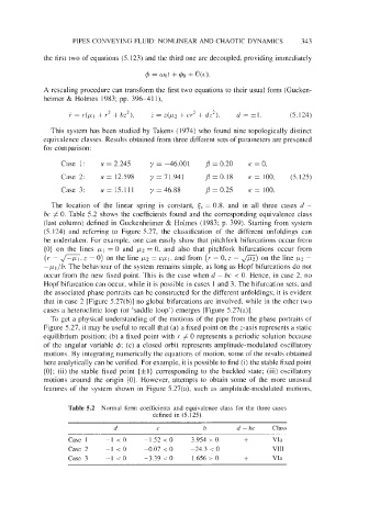
Table 5.2 Normal form coefficients and equivalence class for the three cases
defined in (5.125).

d C b d - bc Class
Case 1 -1 (0 -1.52 < 0 3.954 > 0 + VIa
Case 2 -1 <o -0.07 < 0 -24.3 < 0 - VI11
Case 3 -1 to -3.39 i 1.656 > 0 + VIa
0