Page 370 - Fluid-Structure Interactions Slender Structure and Axial Flow (Volume 1)

350 SLENDER STRUCTURES AND AXIAL FLOW

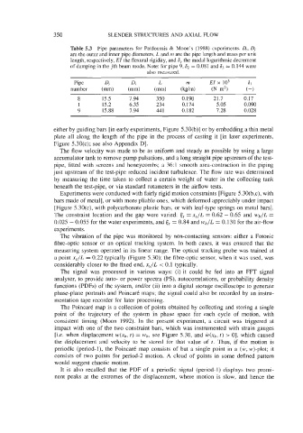
Table 5.3 Pipe parameters for Pdidoussis & Moon’s (1988) experimenls. Do, D;
are the outer and inner pipe diameters, L and m are the pipe length and mass per unit
length, respectively, E1 the flexural rigidity, and 6, the modal logarithmic decrement
of damping in the jth beam mode. Note: for pipe 9, S2 = 0.081 and 63 = 0.144 were
also measured.
Pipe Do D, L m EI x 103 61
number (mm) (mm) (mm) (kg/m) (N m2) (-1
8 15.5 7.94 350 0.190 21.7 0.17
1 15.2 6.35 234 0.174 5.05 0.090
9 15.88 7.94 44 1 0.182 7.28 0.028

either by guiding bars [in early experiments, Figure 5.30(b)] or by embedding a thin metal
plate all along the length of the pipe in the process of casting it [in later experiments,
Figure 5.30(c); see also Appendix D].
The flow velocity was made to be as uniform and steady as possible by using a large
accumulator tank to remove pump pulsations, and a long straight pipe upstream of the test-
pipe, fitted with screens and honeycombs; a 36:l smooth area-contraction in the piping
just upstream of the test-pipe reduced incident turbulence. The flow rate was determined
by measuring the time taken to collect a certain weight of water in the collecting tank
beneath the test-pipe, or via standard rotameters in the airflow tests.
Experiments were conducted with fairly rigid motion constraints [Figure 5.30(b,c), with
bars made of metal], or with more pliable ones, which deformed appreciably under impact
[Figure 5.30(c), with polycarbonate plastic bars, or with leaf-type springs on metal bars].
The constraint location and the gap were varied: tS = n,/L = 0.62 - 0.65 and wb/L =
0.025 - 0.055 for the water experiments, and & = 0.84 and wb/L = 0.130 for the air-flow
experiments.
The vibration of the pipe was monitored by non-contacting sensors: either a Fotonic
fibre-optic sensor or an optical tracking system. In both cases, it was ensured that the
measuring system operated in its linear range. The optical tracking probe was trained at
a point x,/L = 0.22 typically (Figure 5.30); the fibre-optic sensor, when it was used, was
considerably closer to the fixed end, x,/L < 0.1 typically.
The signal was processed in various ways: (i) it could be fed into an FFT signal
analyser, to provide auto- or power spectra (PS), autocorrelations, or probability density
functions (PDFs) of the system, andor (ii) into a digital storage oscilloscope to generate
phase-plane portraits and Poincark maps; the signal could also be recorded by an instru-
mentation tape recorder for later processing.
The Poincare map is a collection of points obtained by collecting and storing a single
point of the trajectory of the system in phase space for each cycle of motion, with
consistent timing (Moon 1992). In the present experiment, a circuit was triggered at
impact with one of the two constraint bars, which was instrumented with strain gauges
[Le. when displacement ~(q,, t) = Wb, see Figure 5.30, and W(xb, t) > 01, which caused
the displacement and velocity to be stored for that value of t. Thus, if the motion is
periodic (period-I), the Poincark map consists of but a single point in a (W, w)-plot; it
consists of two points for period-2 motion. A cloud of points in some defined pattern
would suggest chaotic motion.
It is also recalled that the PDF of a periodic signal (period-1) displays two promi-
nent peaks at the extremes of the displacement, where motion is slow, and hence the