Page 423 - Fluid-Structure Interactions Slender Structure and Axial Flow (Volume 1)

PIPES CONVEYING FLUID: NONLINEAR AND CHAOTIC DYNAMICS 395

In all cases but the first, the pipe is considered to have absolutely fixed ends, i.e. no
axial sliding is permitted, and hence the nonlinear equation of motion used is similar to
Holmes’ and relatively simple, as discussed in what follows. In the case of Yoshizawa
et al. (1986), however, the downstream end of the clamped-pinned pipe considered is free
to slide axially. The equations of motion, similar to Rousselet & Henmann’s (1981), are
much more complex: one ‘flow equation’, similar to those discussed in Section 5.2.8(b,c),
in which the pressure itself is pulsatile, p = pg(1 + p sin wt),+ and an equation for the
pipe coupled to the first, in which nonlinearities are associated with curvature rather
than induced-tension effects, similar to equation (5.43) for cantilevered pipes. This work,
being the first to be published and the simplest in terms of methods used, is discussed
first. The eigenfunctions +,(c) of the subsystem ij + q”” - y[(l - 6)q” - q’] + uiq” = 0
are obtained first, and then the system is discretized via a one-mode Galerkin scheme,
so that ~(6, t) = &(t)q(t), leading to two fairly simple nonlinear coupled ODES in u(t)
and q(t), involving ug, p, PO, j3 and y. Solution of these equations is obtained by the
method of multiple scales (Nayfeh & Mook 1979), and the deflection of the pipe is
finally expressed as q(6, t) = pl/’h cos[;(wt + @)]+,(s) + S(p3/’), in which it has been
assumed that w is close to 2w1, 01 being the first-mode eigenfrequency associated with
+I({). Hence, the first-mode principal parametric resonance is considered (Section 4.3,
involving the ‘detuning parameter’ 3, such that w/wl = 2(1 + pL?).$
A number of interesting findings are reported, as follows. (i) Considering no pulsation,
the mean-flow nonlinear first-mode eigenfrequency plotted in a ui versus y plot shows
both softening and hardening spring characteristics, the former for low ui when inertial
nonlinearities are predominant, the latter for larger ui when nonlinear centrifugal effects
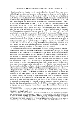
are dominant. (ii) The steady-state amplitude, h,, associated with p1I2h in the foregoing, is
determined and its stability examined, eventually producing the classical plot of h, versus
0 = p13 shown in Figure 5.59(a). It is clear that as p becomes larger, since p < 1, both h,
and 0 increase - i.e. the frequency range and amplitude increase with p. (iii) The extent
of the parametric resonance region is larger in terms of 0 than the linear range, because of
the subcritical onset of the oscillation with decreasing 6, leading to hysteresis (hardening
behaviour) as seen in Figure 5.59(a). (iv) The maximum amplitude increases with ug.
Experiments have also been done by Yoshizawa etal. (1985, 1986) using silicone
rubber pipes (0, = 5 mm, L = 600 mm) stiffened in one plane by wires, to confine the
oscillation in the other plane - see also Section 5.5.3. The pulsation was introduced
by periodic opening and shutting of a pressure-control valve at the exit of a by-pass
line connected to the constant-head tank feeding water into the pipe. The experimental
results are in good qualitative agreement with theory. Figure 5.59(b-d) shows the pipe
in parametric resonance as 0 is increased, i.e. as the pulsation frequency is increased,
showing that the amplitude increases. For 0 = 0.183 (not shown), the amplitude begins
to decrease and soon thereafter the oscillation ceases. The oscillation if excited at or

tThroughout Section 5.9, p denotes the amplitude of harmonic perturbations, usually of the flow velocity.
as in Section 4.5 - see equation (5.144). It should not be confused with the dimensionless end-mass parameter
in equation (5.139) used in Section 5.8.3.
$It is recalled that, in order to achieve a modicum of uniformity in the book, the notation is sometimes
quite different from that in the original papers - though this may be bewildering to their authors! Especially in
the case of the detuning parameter, since different definitions are given in virtually every study, the following
convention has been used: (i) if the detuning parameter is multiplied by a small parameter, it is denoted by 6.
and
as in Yoshizawa et al. (1986) where W/WI = 2(1 + ~6) Bajaj (1987b) where w = OAJ - €6; (ii) otherwise.
it is denoted by 5, as in equation (5.148) where w/wg = 1 - 5, and in Bajaj (1984) where w = wg - 0.