Page 547 - Fluid-Structure Interactions Slender Structure and Axial Flow (Volume 1)

THE FRACTAL DIMENSION FROM THE EXPERIMENTAL PIPE-VIBRATION 5 17

The main problem that must be addressed in applying equations (1.1) and (1.2) to
experimental data is that the data record (e.g. the sampled output from the optical tracking
system in Figure 5.30) is of the form

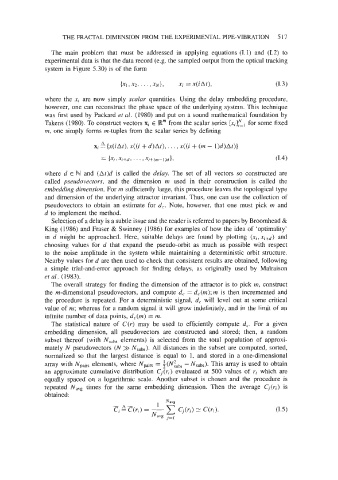
where the xi are now simply scalar quantities. Using the delay embedding procedure,
however, one can reconstruct the phase space of the underlying system. This technique
was first used by Packard et al. (1980) and put on a sound mathematical foundation by
Takens (1 980). To construct vectors xi E R" from the scalar series [xi& for some fixed
m, one simply forms m-tuples from the scalar series by defining

x, {x(iAt), x((i + d)Af), . . . , x((i + (m - l)d)At)}
= {xi, xi+d. . . * I Xi+(m-l)dJ, (1.4)

where d E N and (At)d is called the delay. The set of all vectors so constructed are
called pseudovectors, and the dimension m used in their construction is called the
embedding dimension. For m sufficiently large, this procedure leaves the topological type
and dimension of the underlying attractor invariant. Thus, one can use the collection of
pseudovectors to obtain an estimate for d,. Note, however, that one must pick m and
d to implement the method.
Selection of a delay is a subtle issue and the reader is referred to papers by Broomhead &
King (1986) and Fraser & Swinney (1986) for examples of how the idea of 'optimality'
in d might be approached. Here, suitable delays are found by plotting (xi,xi+d) and
choosing values for d that expand the pseudo-orbit as much as possible with respect
to the noise amplitude in the system while maintaining a deterministic orbit structure.
Nearby values for d are then used to check that consistent results are obtained, following
a simple trial-and-error approach for finding delays, as originally used by Malraison
et al. (1983).
The overall strategy for finding the dimension of the attractor is to pick m, construct
the m-dimensional pseudovectors, and compute d, = d,(m); m is then incremented and
the procedure is repeated. For a deterministic signal, d, will level out at some critical
value of m; whereas for a random signal it will grow indefinitely, and in the limit of an
infinite number of data points, d,(m) = m.
The statistical nature of C(r) may be used to efficiently compute d,. For a given
embedding dimension, all pseudovectors are constructed and stored; then, a random
subset thereof (with Nsubs elements) is selected from the total population of approxi-
mately N pseudovectors (N >> Nsubs). All distances in the subset are computed, sorted,
normalized so that the largest distance is equal to 1, and stored in a one-dimensional
array with Npairs elements, where Npirs = i(N:ubs - Nsubs). This array is used to obtain
an approximate cumulative distribution C,(ri) evaluated at 500 values of ri which are
equally spaced on a logarithmic scale. Another subset is chosen and the procedure is
repeated Nav, times for the same embedding dimension. Then the average Cj(ri) is
obtained: