Page 548 - Fluid-Structure Interactions Slender Structure and Axial Flow (Volume 1)

518 SLENDER STRUCTURES AND AXIAL FLOW

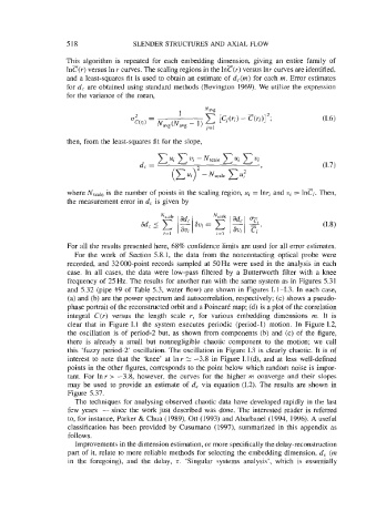
This algorithm is repeated for each embedding dimension, giving an entire family of
Inc(r) versus In r curves. The scaling regions in the lnC(r) versus lnr curves are identified,
and a least-squares fit is used to obtain an estimate of d,(m) for each m. Error estimates
for d, are obtained using standard methods (Bevington 1969). We utilize the expression
for the variance of the mean,

then, from the least-squares fit for the slope,

(7.7)

where Nscde is the number of points in the scaling region, ui = lnri and wi = lnci. Then,
the measurement error in d, is given by

For all the results presented here, 68% confidence limits are used for all error estimates.
For the work of Section 5.8.1, the data from the noncontacting optical probe were
recorded, and 32 000-point records sampled at 50 Hz were used in the analysis in each
case. In all cases, the data were low-pass filtered by a Buttenvorth filter with a knee
frequency of 25 Hz. The results for another run with the same system as in Figures 5.31
and 5.32 (pipe #I9 of Table 5.3, water flow) are shown in Figures 1.1-1.3. In each case,
(a) and (b) are the power spectrum and autocorrelation, respectively; (c) shows a pseudo-
phase portrait of the reconstructed orbit and a Poincark map; (d) is a plot of the correlation
integral C(r) versus the length scale r, for various embedding dimensions m. It is
clear that in Figure 1.1 the system executes periodic (period-1) motion. In Figure 1.2,
the oscillation is of period-2 but, as shown from components (b) and (c) of the figure,
there is already a small but nonnegligible chaotic component to the motion; we call
this ‘fuzzy period-2’ oscillation. The oscillation in Figure 1.3 is clearly chaotic. It is of
interest to note that the ‘knee’ at Inr 2: -3.8 in Figure I.l(d), and at less well-defined
points in the other figures, corresponds to the point below which random noise is impor-
tant. For lnr > -3.8, however, the curves for the higher m converge and their slopes
may be used to provide an estimate of d, via equation (1.2). The results are shown in
Figure 5.37.
The techniques for analysing observed chaotic data have developed rapidly in the last
few years - since the work just described was done. The interested reader is referred
to, for instance, Parker & Chua (1989), Ott (1993) and Abarbanel (1994, 1996). A useful
classification has been provided by Cusumano (1997), summarized in this appendix as
follows.
Improvements in the dimension estimation, or more specifically the delay-reconstruction
part of it, relate to more reliable methods for selecting the embedding dimension, d, (m
in the foregoing), and the delay, t. ‘Singular systems analysis’, which is essentially