
Page 71 - Fluid-Structure Interactions Slender Structure and Axial Flow (Volume 1)
P. 71
54 SLENDER STRUCTURES AND AXIAL FLOW
Physically, flutter is a self-excited oscillation, which grows from sensibly zero to a
steady oscillation of finite amplitude and constant frequency, thus to a closed curve
in the phase plane (x,X), i.e. to a limit cycle. Mathematically, the onset of flutter is
characterized by a pair of eigenvalues crossing from %e(A) < 0 to %e(A) > 0 as U
is increased, such that at U = U, (i) the pair is purely imaginary, i.e. %e(a) = 0, and
(ii) 9am(A) # 0 [Figure 2.10(b)]. This is defined as a Hopf bifurcation. In many cases,
the evolution in the phase plane as U is increased is as shown in three-dimensional
form in Figure 2.11(b), in which case the Hopf bifurcation is supercritical. As shown
in Figure 2.1 l(c), the origin has become unstable and oscillatory solutions of a certain
amplitude are possible for U > U,. If the system is perturbed, it will eventually settle
down on the limit cycle; hence this is a case of a stable limit cycle.
A subcritical Hopf bifurcation is illustrated in Figure 2.1 1 (d), where the limit cycle
generated is unstable or ‘repelling’; as shown by the small arrows, oscillatory solutions
either die out to the stable equilibrium (stable fixed point) or diverge to larger amplitudes.
In real physical systems, the existence of this unstable limit cycle usually implies that
a stable ‘attracting’ one [as shown in Figure 2.11(d)] or another kind of stable solution
exists at larger amplitudes; so that, the trajectories in the phase plane, repelled by the
unstable limit cycle, will gravitate towards the stable fixed (equilibrium) point or the
limit cycle beyond. Thus, the system is then said to be unstable in the small, but stable
in the large. A more formal definition of stability is given in Appendix F.l.l.
The behaviour described in the foregoing may be illustrated by a fictitious nonlinear
one-degree-of-freedom system, the equation of motion of which is
mx + cg(X) + kf(x) = 0, (2.164)
and which may be viewed as a nonlinear version of equation (2.160) for a specific value
of U; g(i) and f(x) are nonlinear functions. As it is not uncommon for these functions to
be odd, let us illustrate the behaviour of such a system by the following particular case:
2 + 0.02( 1 - X2)i + (1 - 0.02x2)x = 0. (2.165)
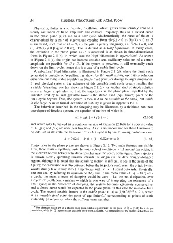
Trajectories in the phase plane are shown in Figure 2.12. Two main features are visible.
First, there exists a repelling, unstable limit cycle of amplitude - 1.1 around the origin, in
the clear white oval between the darker patches near the centre of the figure. One trajectory
is shown, slowly spiralling inwards towards the origin (in the dark doughnut-shaped
region, although it is noted that the spiralling motion is difficult to see in the scale of the
figure); the calculation was discontinued before the trajectory could reach the origin (which
would strictly take infinite time). Trajectories with 1x1 > 1.1 spiral outwards. Physically,
one can see, by referring to equation (2.165), that if the mean value of 1i-l - O(1) over
a cycle, the mean amount of damping would be zero - i.e. the net dissipation, over
a cycle of oscillation, vanishes - which is one way of interpreting the existence of a
limit cycle; in the ‘absence’ of damping, the system becomes efectively conservative,
and a closed curve would be expected in the phase plane, in this case the unstable limit
cycle. The second notable feature is the saddle point at 1x1 = (1/0.02)1/2 2 7.1, which
is an unstable fied point (or point of equilibrium),’ corresponding to points of static
instability (divergence), when the stiffness term vanishes.
t The classical paradigm of a stable fixed point (stable equilibrium) is the point (0, 6) = (0,O) for a simple
pendulum. while (IT, 0) represents an unstable fixed point, a saddle. A characteristic of the saddle is that there are