
Page 72 - Fluid-Structure Interactions Slender Structure and Axial Flow (Volume 1)
P. 72
CONCEPTS, DEFINITIONS AND METHODS 55
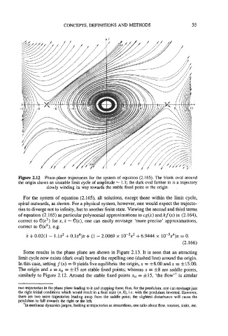
Figure 2.12 Phase-plane trajectories for the system of equation (2.165). The blank oval around
the origin shows an unstable limit cycle of amplitude - 1.1; the dark oval farther in is a trajectory
slowly winding its way towards the stable fixed point at the origin.
For the system of equation (2.165), all solutions, except those within the limit cycle,
spiral outwards, as shown. For a physical system, however, one would expect the trajecto-
ries to diverge not to infinity, but to another finite state. Viewing the second and third terms
of equation (2.165) as particular polynomial approximations to cg(x) and kf(x) in (2.164),
correct to O(e3) for x, .i - 6(r), one can easily envisage 'more precise' approximations,
correct to S(e5), e.g.
i + 0.02~ - i.ii2 + 0.1i4)i + (1 - 2.0069 io-2x2 + 6.9444 10-%~)~ 0.
=
(2.166)
Some results in the phase plane are shown in Figure 2.13. It is seen that an attracting
limit cycle now exists (dark oval) beyond the repelling one (dashed line) around the origin.
In this case, setting f(x) = 0 yields five equilibria: the origin, x = f8.00 and x = f15.00.
The origin and x = xst = f15 are stable fixed points; whereas x = f8 are saddle points,
similarly to Figure 2.12. Around the stable fixed points xst = f15, 'the flow" is similar
two trajectories in the phase plane leading to it and stopping there; thus, for the pendulum, one can envisage just
the right initial conditions which would result in a final state (n. 01, Le. with the pendulum inverted. However,
there are two more trajectories leading away from the saddle point; the slightest disturbance will cause the
pendulum to fall towards the right or the left.
'In nonlinear dynamics jargon, looking at trajectories as streamlines, one talks about flow, sources, sinks, etc.