Page 135 - T. Anderson-Fracture Mechanics - Fundamentals and Applns.-CRC (2005)

1656_C003.fm Page 115 Monday, May 23, 2005 5:42 PM

Elastic-Plastic Fracture Mechanics 115

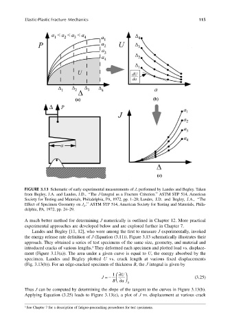
FIGURE 3.13 Schematic of early experimental measurements of J, performed by Landes and Begley. Taken
from Begley, J.A. and Landes, J.D., ‘‘The J-Integral as a Fracture Criterion.’’ ASTM STP 514, American
Society for Testing and Materials, Philadelphia, PA, 1972, pp. 1–20; Landes, J.D. and Begley, J.A., ‘‘The
Effect of Specimen Geometry on J Ic .’’ ASTM STP 514, American Society for Testing and Materials, Phila-
delphia, PA, 1972, pp. 24–29.

A much better method for determining J numerically is outlined in Chapter 12. More practical
experimental approaches are developed below and are explored further in Chapter 7.
Landes and Begley [11, 12], who were among the first to measure J experimentally, invoked
the energy release rate definition of J (Equation (3.11)). Figure 3.13 schematically illustrates their
approach. They obtained a series of test specimens of the same size, geometry, and material and
3
introduced cracks of various lengths. They deformed each specimen and plotted load vs. displace-
ment (Figure 3.13(a)). The area under a given curve is equal to U, the energy absorbed by the
specimen. Landes and Begley plotted U vs. crack length at various fixed displacements
(Fig. 3.13(b)). For an edge-cracked specimen of thickness B, the J integral is given by

J =− 1   ∂ U   (3.25)
B ∂  ∆

a
Thus J can be computed by determining the slope of the tangent to the curves in Figure 3.13(b).
Applying Equation (3.25) leads to Figure 3.13(c), a plot of J vs. displacement at various crack

3 See Chapter 7 for a description of fatigue-precracking procedures for test specimens.