Page 377 - T. Anderson-Fracture Mechanics - Fundamentals and Applns.-CRC (2005)

1656_C008.fm Page 357 Monday, May 23, 2005 5:59 PM

Fracture Testing of Nonmetals 357

EXAMPLE 8.1

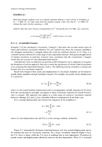
Short-time fracture toughness tests on a polymer specimen indicate a crack velocity of 10 mm/sec at
K Ic = 5 MPa m . If a pipe made from this material contains a flaw such that K I = 2.5 MPa m ,
estimate the crack velocity, assuming n = 0.08.

12.5
Solution: Since the crack velocity is proportional to K I , the growth rate at 2.5 MPa m is given by
 . 25 MPa m  12 .5
˙ a = 10 mm /sec   = . 0 0017 mm /sec = . 6 2 mm/h
 5 MPa m 

8.1.1.2 J-Controlled Fracture

Schapery [1,2] has introduced a viscoelastic J integral J that takes into account various types of
v
linear and nonlinear viscoelastic behavior. For any material that obeys the assumed constitutive
law, Schapery showed that J uniquely defines the crack-tip conditions (Section 4.3.2). Thus, J is
v
v
a suitable fracture criterion for a wide range of time-dependent materials. Most practical applications
of fracture mechanics to polymers, however, have considered only the conventional J integral,
which does not account for time-dependent deformation.
Conventional J tests on polymers can provide useful information, but is important to recognize
the limitations of such an approach. One way to assess the significance of critical J data for polymers
is by evaluating the relationship between J and J . The following exercise considers a constant rate
v
fracture test on a viscoelastic material.
Recall from Chapter 4 that strains and displacements in viscoelastic materials can be related to
pseudo-elastic quantities through hereditary integrals. For example, the pseudo-elastic displacement
e
∆ is given by

∆ = e E R −1 ∫ t E ( t − ∂ ∆ d) τ τ (8.10)
0 ∂τ
where ∆ is the actual load-line displacement and τ is an integration variable. Equation (8.10) stems
from the correspondence principle, and applies to linear viscoelastic materials for which Poisson’s
ratio is constant. This approach also applies to a wide range of nonlinear viscoelastic material
behavior, although E(t) and E have somewhat different interpretations in the latter case.
R
For a constant displacement rate fracture test, Equation (8.10) simplifies to

∆ e ∆ = ˙ E −1 ∫ t E ( t ) ττ
d −
R
0
=∆ Et () (8.11)
E R
˙
∆
where is the displacement rate and Et() is a time-average modulus, defined by
Et() = 1 ∫ t Et − ( d ) τ τ (8.12)
t 0

Figure 8.3 schematically illustrates load-displacement and load pseudo-displacement curves
for constant rate tests on viscoelastic materials. For a linear viscoelastic material (Figure 8.3(a)),
e
the P-∆ curve is linear, while the P-∆ curve is nonlinear due to time dependence. Evaluation of
e
pseudo strains and displacements effectively removes the time dependence. When ∆ is evaluated