Page 117 - Fundamentals of Communications Systems

Review of Probability and Random Variables 3.31

(b) What is P (C)?
(c) What is the P (A and C) = P (A∩ C)?
(d) Compute P (A|C).
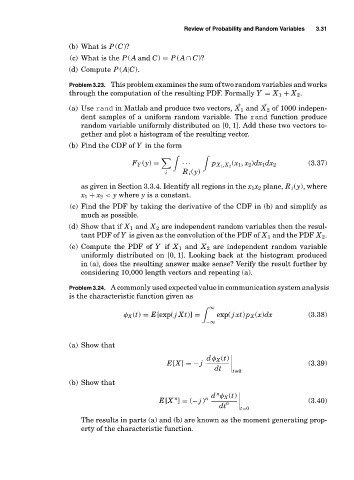
Problem 3.23. This problem examines the sum of two random variables and works
through the computation of the resulting PDF. Formally Y = X 1 + X 2 .
(a) Use rand in Matlab and produce two vectors, X 1 and X 2 of 1000 indepen-

dent samples of a uniform random variable. The rand function produce
random variable uniformly distributed on [0, 1]. Add these two vectors to-
gether and plot a histogram of the resulting vector.
(b) Find the CDF of Y in the form

F Y (y) = ··· p X 1 ,X 2 (x 1 , x 2 )dx 1 dx 2 (3.37)
i R i (y)
as given in Section 3.3.4. Identify all regions in the x 1 x 2 plane, R i (y), where
x 1 + x 2 < y where y is a constant.
(c) Find the PDF by taking the derivative of the CDF in (b) and simplify as
much as possible.
(d) Show that if X 1 and X 2 are independent random variables then the resul-
tant PDF of Y is given as the convolution of the PDF of X 1 and the PDF X 2 .
(e) Compute the PDF of Y if X 1 and X 2 are independent random variable
uniformly distributed on [0, 1]. Looking back at the histogram produced
in (a), does the resulting answer make sense? Verify the result further by
considering 10,000 length vectors and repeating (a).

Problem 3.24. A commonly used expected value in communication system analysis
is the characteristic function given as
∞

φ X (t) = E[exp( jXt)] = exp( jxt) p X (x)dx (3.38)
−∞

(a) Show that

dφ X (t)
E[X] =− j (3.39)
dt
t=0
(b) Show that
n
n
E[X ] = (− j ) n d φ X (t) (3.40)
n
dt
t=0
The results in parts (a) and (b) are known as the moment generating prop-
erty of the characteristic function.