Page 61 - Fundamentals of Communications Systems

Signals and Systems Review 2.13

0 −30
−5 −35
−10 −40
−15 −45
G x (f), dB −25 G x (f), dB −50
−20
−55
−30
−35 −60
−65
−40 −70
−45 −75
−50 −80
0 5 10 15 20 25 30 35 40 −5000 −3000 −1000 0 1000 3000 5000
Normalized Frequency, fT p Frequency, f, Hz
(a) Pulse (b) ‘Bingo’ Signal
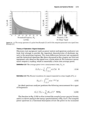
Figure 2.3 (a) The energy spectrum of a pulse from Example 2.1 and (b) the computer-generated voice signal from
Example 2.3.

Theory of Operation: Signal Analyzers
Electronic test equipment (such as power meters and spectrum analyzers) are
tools that attempt to provide the important characteristics of electronic sig-
nals to the practicing engineer. The main differences between test equipment
and the theoretical equations like those discussed in this chapter are that test
equipment only observes the signal over a finite interval. For instance a power
meter outputs a reading, which is essentially a finite time average power.
Definition 2.8 The average power over a measurement time, T m ,is

T m /2

1 2
P x (T m ) = |x(t)| dt W (2.54)
T m
−T m /2
Definition 2.9 The Fourier transform of a signal truncated to a time length of T m is
T m /2

(f ) = x(t)e − j 2π ft dt (2.55)
X T m
−T m /2
An ideal spectrum analyzer produces the following measurement for a span
of frequencies

1 2
S x ( f , T m ) = |X T m (f )| W/Hz (2.56)
T m
The function in Eq. (2.56) is often termed the sampled power spectral density
and it is a direct analog to the energy spectral density of Eq. (2.47). The sampled
power spectrum is a functional description of how the power in the truncated