Page 66 - Fundamentals of Communications Systems

2.18 Chapter Two

B 40 = 152/T , and B 98 = 26/T . Note the computation of B 98 required a Matlab program
to be written to sum the magnitude square of the Fourier series coefficients. B 40 can
only be identified by expanding the x-axis in Figure 2.4 as the spectrum has not yet gone
40 dB down in this figure.

2.2.5 Laplace Transforms
This text will use the one-sided Laplace transform for the analysis of tran-
sient signals in communications systems. The one–sided Laplace transform of
a signal x(t)is
∞

X(s) = L{x(t)}= x(t) exp[−st]dt (2.69)
0
The use of the one-sided Laplace transform implies that the signal is zero for
negative time. The inverse Laplace transform is given as
1
x(t) = X(s) exp[st]ds (2.70)
2π j
The evaluation of the general inverse Laplace transform requires the evalu-
ation of contour integrals in the complex plane. For most transforms of interest
the results are available in tables.

EXAMPLE 2.28
2π f m
x(t) = sin(2π f m t) X(s) =
2
s + (2π f m ) 2
s
x(t) = cos(2π f m t) X(s) =
2
s + (2π f m ) 2
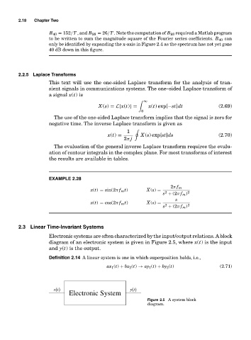
2.3 Linear Time-Invariant Systems

Electronic systems are often characterized by the input/output relations. A block
diagram of an electronic system is given in Figure 2.5, where x(t) is the input
and y(t) is the output.

Definition 2.14 A linear system is one in which superposition holds, i.e.,
ax 1 (t) + bx 2 (t) → ay 1 (t) + by 2 (t) (2.71)

xt () yt ()
Electronic System
Figure 2.5 A system block
diagram.