Page 70 - Fundamentals of Communications Systems

2.22 Chapter Two

EXAMPLE 2.31
Consider the signal from Example 2.1, x(t) = cos(2π f m t) input into an arbitrary filter
characterized with a transfer function H(f ). The output Fourier series coefficients are
H( f m ) H(− f m )
f T = f m y 1 = y −1 = x n = 0 (2.77)
2 2
and denoting the amplitude of the transfer funtion with H A (f ) and the phase of the
transfer function with H P (f ) the output signal is
y(t) = H A ( f m ) cos(2π f m t + H P ( f m )) (2.78)

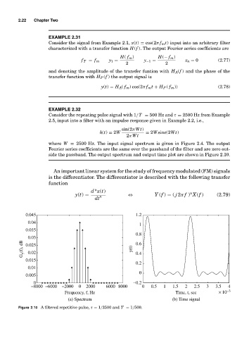
EXAMPLE 2.32
Consider the repeating pulse signal with 1/T = 500 Hz and τ = 2500 Hz from Example
2.5, input into a filter with an impulse response given in Example 2.2, i.e.,

sin(2πWt)
h(t) = 2W = 2Wsinc(2Wt)
2πWt
where W = 2500 Hz. The input signal spectrum is given in Figure 2.4. The output
Fourier series coefficients are the same over the passband of the filter and are zero out-
side the passband. The output spectrum and output time plot are shown in Figure 2.10.

An important linear system for the study of frequency modulated (FM) signals
is the differentiator. The differentiator is described with the following transfer
function
n
d x(t) n
y(t) = n ⇔ Y (f ) = ( j 2π f ) X(f ) (2.79)
dt

0.045 1.2
0.04
1
0.035
0.8
0.03
G y (f), dB 0.025 y(t) 0.6

0.02
0.4
0.015
0.2
0.01
0
0.005
0 −0.2
−8000 −6000 −2000 0 2000 6000 8000 0 0.5 1 1.5 2 2.5 3 3.5 4
Frequency, f, Hz Time, t, sec × 10 −3
(a) Spectrum (b) Time signal
Figure 2.10 A filtered repetitive pulse, τ = 1/2500 and T = 1/500.