
Page 82 - Fundamentals of Communications Systems
P. 82
2.34 Chapter Two
10
5
x(t) 0
−5
−10
0 0.01 0.02 0.03 0.04 0.05 0.06 0.07 0.08
10
5
x(t) 0
−5
−10
0 0.01 0.02 0.03 0.04 0.05 0.06 0.07 0.08
10
5
x(t) 0
−5
−10
0 0.01 0.02 0.03 0.04 0.05 0.06 0.07 0.08
Time, t, sec
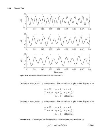
Figure 2.16 Plots of the time waveforms for Problem 2.2.
(b) x(t) = 2 cos(200πt) + 5 sin(300πt). The waveform is plotted in Figure 2.16.
1 = 50 x 2 = 1 x −2 = 1
T
T = 0.02 x 3 = 5 x −3 = −5
j 2 j 2
x n = 0 otherwise
(c) x(t) = 2 cos(150πt) + 5 sin(250πt). The waveform is plotted in Figure 2.16.
1 = 25 x 3 = 1 x −3 = 1
T
T = 0.04 x 5 = 5 x −5 = −5
j 2 j 2
x n = 0 otherwise
Problem 2.25. The output of the quadratic nonlinearity is modeled as
2
y(t) = ax(t) + bx (t) (2.104)