
Page 77 - Fundamentals of Communications Systems
P. 77
Signals and Systems Review 2.29
(a) Compute X(f ).
(b) Compute E x .
dx(t)
(c) Compute y(t) = .
dt
(d) Compute Y (f ).
Hint: Some of the computations have an easy way and a hard way so think
before turning the crank!
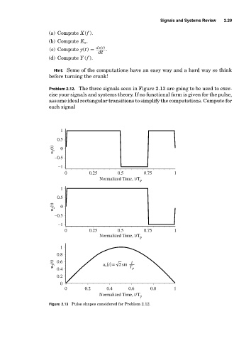
Problem 2.12. The three signals seen in Figure 2.13 are going to be used to exer-
cise your signals and systems theory. If no functional form is given for the pulse,
assume ideal rectangular transitions to simplify the computations. Compute for
each signal
1
0.5
u 1 (t) 0
−0.5
−1
0 0.25 0.5 0.75 1
Normalized Time, t/T p
1
0.5
u 2 (t) 0
−0.5
−1
0 0.25 0.5 0.75 1
Normalized Time, t/T p
1
0.8
u 3 (t) 0.6 ut() = 2 sin t
3
0.4 T p
0.2
0
0 0.2 0.4 0.6 0.8 1
Normalized Time, t/T p
Figure 2.13 Pulse shapes considered for Problem 2.12.