Page 95 - Fundamentals of Communications Systems

Review of Probability and Random Variables 3.9

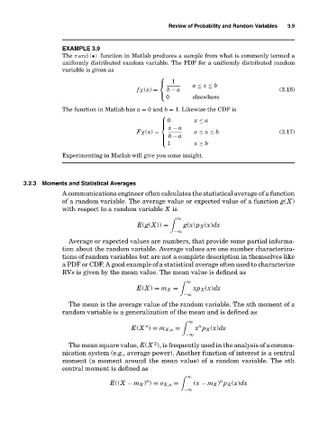
EXAMPLE 3.9
The rand(•) function in Matlab produces a sample from what is commonly termed a
uniformly distributed random variable. The PDF for a uniformly distributed random
variable is given as
⎧
1
a ≤ x ≤ b
⎨
f X (x) = b − a (3.16)
0 elsewhere
⎩
The function in Matlab has a = 0 and b = 1. Likewise the CDF is
⎧
⎪ 0 x ≤ a
⎪
x − a
⎨
F X (x) = a ≤ x ≤ b (3.17)
⎪ b − a
⎪
1 x ≥ b
⎩
Experimenting in Matlab will give you some insight.
3.2.3 Moments and Statistical Averages
A communications engineer often calculates the statistical average of a function
of a random variable. The average value or expected value of a function g(X)
with respect to a random variable X is

∞
E(g(X)) = g(x) p X (x)dx
−∞
Average or expected values are numbers, that provide some partial informa-
tion about the random variable. Average values are one number characteriza-
tions of random variables but are not a complete description in themselves like
a PDF or CDF. A good example of a statistical average often used to characterize
RVs is given by the mean value. The mean value is defined as
∞

E(X) = m X = xp X (x)dx
−∞
The mean is the average value of the random variable. The nth moment of a
random variable is a generalization of the mean and is defined as
∞

n n
E(X ) = m X,n = x p X (x)dx
−∞
2
The mean square value, E(X ), is frequently used in the analysis of a commu-
nication system (e.g., average power). Another function of interest is a central
moment (a moment around the mean value) of a random variable. The nth
central moment is defined as
∞

n n
E((X − m X ) ) = σ X,n = (x − m X ) p X (x)dx
−∞