Page 97 - Fundamentals of Communications Systems

Review of Probability and Random Variables 3.11

0.4 0.8
0.35 0.7 Variance = 0.25
0.3 mean = 0 mean = 1 0.6
0.25 0.5
f X (x) 0.2 f X (X) 0.4
0.15 0.3 Variance = 1

0.1 0.2
Variance = 4
0.05 0.1
0 0
−5 −4 −3 −2 −1 0 1 2 3 4 5 −5 −4 −3 −2 −1 0 1 2 3 4 5
x x
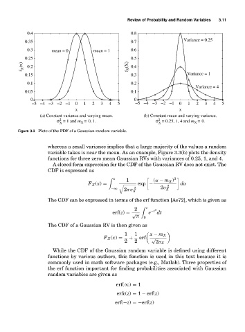
(a) Constant variance and varying mean. (b) Constant mean and varying variance.
2
2
σ = 1 and m = 0, 1. σ = 0.25, 1, 4 and m = 0.
X X X X
Figure 3.3 Plots of the PDF of a Gaussian random variable.
whereas a small variance implies that a large majority of the values a random
variable takes is near the mean. As an example, Figure 3.3(b) plots the density
functions for three zero mean Gaussian RVs with variances of 0.25, 1, and 4.
A closed form expression for the CDF of the Gaussian RV does not exist. The
CDF is expressed as

x
1 (α − m X )
2
F X (x) = exp − 2 dα
2πσ X
−∞ 2 2σ X
The CDF can be expressed in terms of the erf function [Ae72], which is given as
2 z −t 2
erf(z) = √ e dt
π 0
The CDF of a Gaussian RV is then given as
1 1 x − m X
F X (x) = + erf √
2 2 2σ X
While the CDF of the Gaussian random variable is defined using different
functions by various authors, this function is used in this text because it is
commonly used in math software packages (e.g., Matlab). Three properties of
the erf function important for finding probabilities associated with Gaussian
random variables are given as

erf(∞) = 1
erfc(z) = 1 − erf(z)

erf(−z) =−erf(z)