Page 98 - Fundamentals of Communications Systems

3.12 Chapter Three

EXAMPLE 3.11
The randn(•) function in Matlab produces a sample from a Gaussian distributed ran-
dom variable with m X = 0 and σ X = 1.

3.2.5 A Transformation of a Random Variable
In the analysis of communication system performance it is often necessary to
characterize a random variable, which is a transformation of another random
variable. This transformation is expressed as

Y = g(X)
This section is concerned with finding the PDF or the CDF of the random
variable, Y . The general technique is a two step process.

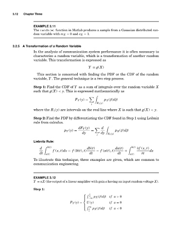
Step 1: Find the CDF of Y as a sum of integrals over the random variable X
such that g(X) < y. This is expressed mathematically as

F Y (y) = p X (β)dβ
R i (y)
i
where the R i (y) are intervals on the real line where X is such that g(X) < y.

Step 2: Find the PDF by differentiating the CDF found in Step 1 using Leibniz
rule from calculus.
dF Y (y) d
p Y (y) = = p X (β)dβ
dy dy R i (y)
i
Liebnitz Rule:
d b(t) db(t) da(t) b(t) ∂ f (x, t)
f (x, t)dx = f (b(t), t) − f (a(t), t) + dx
dt a(t) dt dt a(t) ∂t
To illustrate this technique, three examples are given, which are common to
communication engineering.

EXAMPLE 3.12
Y = aX (the output of a linear amplifier with gain a having an input random voltage X).

Step 1:
⎧ y
a p X (β)dβ if a > 0
⎪
⎪ −∞
⎨
F Y (y) = U (y) if a = 0
⎪
⎪ ∞
y p X (β)dβ if a < 0
⎩
a