Page 103 - Fundamentals of Communications Systems

Review of Probability and Random Variables 3.17

0.2

0.15
f XY (x, y) 0.1

0.05

0
4
2 4
2
0
y 0
−2 x
−2
−4 −4
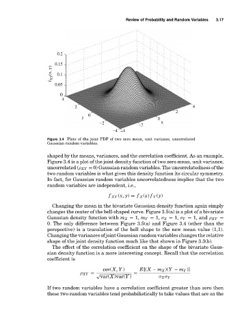
Figure 3.4 Plots of the joint PDF of two zero mean, unit variance, uncorrelated
Gaussian random variables.

shaped by the means, variances, and the correlation coefficient. As an example,
Figure 3.4 is a plot of the joint density function of two zero mean, unit variance,
uncorrelated (ρ XY = 0) Gaussian random variables. The uncorrelatedness of the
two random variables is what gives this density function its circular symmetry.
In fact, for Gaussian random variables uncorrelatedness implies that the two
random variables are independent, i.e.,
f XY (x, y) = f X (x) f Y (y)

Changing the mean in the bivariate Gaussian density function again simply
changes the center of the bell-shaped curve. Figure 3.5(a) is a plot of a bivariate
Gaussian density function with m X = 1, m Y = 1, σ X = 1, σ Y = 1, and ρ XY =
0. The only difference between Figure 3.5(a) and Figure 3.4 (other than the
perspective) is a translation of the bell shape to the new mean value (1,1).
Changing the variances of joint Gaussian random variables changes the relative
shape of the joint density function much like that shown in Figure 3.3(b).
The effect of the correlation coefficient on the shape of the bivariate Gaus-
sian density function is a more interesting concept. Recall that the correlation
coefficient is

cov(X, Y ) E[(X − m X )(Y − m Y )]
ρ XY = √ =
var(X)var(Y ) σ X σ Y
If two random variables have a correlation coefficient greater than zero then
these two random variables tend probabilistically to take values that are on the