Page 104 - Fundamentals of Communications Systems

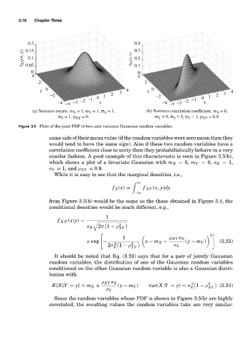
3.18 Chapter Three

0.2 0.4
f XY (x, y) 0.15 f XY (x, y) 0.3
0.1
0.2
0.05
0 0.1
0
4 4
2 2
y 0 3 4 y 0 4
−2 0 1 2 −2 0 1 2 3
−4 −4 −3 −2 −1 x −4 −4 −3 −2 −1 x
(a) Nonzero means. m = 1, m = 1, σ = 1, (b) Nonzero correlation coefficient. m = 0,
Y
X
X
X
σ = 1, ρ XY = 0. m Y = 0, σ = 1, σ = 1, ρ XY = 0.9.
X
Y
Y
Figure 3.5 Plots of the joint PDF of two unit variance Gaussian random variables.
same side of their mean value (if the random variables were zero mean then they
would tend to have the same sign). Also if these two random variables have a
correlation coefficient close to unity then they probabilistically behave in a very
similar fashion. A good example of this characteristic is seen in Figure 3.5(b),
which shows a plot of a bivariate Gaussian with m X = 0, m Y = 0, σ X = 1,
σ Y = 1, and ρ XY = 0.9.
While it is easy to see that the marginal densities, i.e.,
∞

f X (x) = f XY (x, y)dy
−∞
from Figure 3.5(b) would be the same as the those obtained in Figure 3.4, the
conditional densities would be much different, e.g.,

1
f X|Y (x|y) =
2
σ X 2π 1 − ρ XY
2
1 ρ XY σ X
× exp − 2 2 x − m X − (y − m Y ) (3.23)
2σ X 1 − ρ XY σ Y
It should be noted that Eq. (3.23) says that for a pair of jointly Gaussian
random variables, the distribution of one of the Gaussian random variables
conditioned on the other Gaussian random variable is also a Gaussian distri-
bution with
ρ XY σ X 2 2
E[X|Y = y] = m X + (y − m Y ) var(X|Y = y) = σ 1 − ρ (3.24)
X XY
σ Y
Since the random variables whose PDF is shown in Figure 3.5(b) are highly
correlated, the resulting values the random variables take are very similar.