Page 105 - Fundamentals of Communications Systems

Review of Probability and Random Variables 3.19

This is reflected in the knife edge characteristic that the density function takes
along the line Y = X.

3.3.4 Transformations of Random Variables
In general, the problem of finding a probabilistic description (joint CDF or
PDF) of a joint transformation of random variables is very difficult. To simplify
the presentation, two of the most common and practical transformations will
be considered: the single function of n random variables and the one-to-one
transformation.

Single Function of n Random Variables
A single function transformation of n random variables is expressed as

Y = g(X 1 , X 2 , ... , X n )

where X 1 , ... , X n are the noriginal random variables. This section is concerned
with finding the PDF or the CDF of the random variable Y . The general tech-
nique is the identical two step process used for a single random variable (the
regions of integration now become volumes instead of intervals).

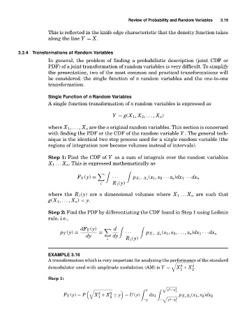
Step 1: Find the CDF of Y as a sum of integrals over the random variables
X 1 ... X n . This is expressed mathematically as

F Y (y) = ··· p X 1 ···X n (x 1 , x 2 ··· x n )dx 1 ··· dx n
i R i (y)
where the R i (y) are n dimensional volumes where X 1 ... X n are such that
g(X 1 , ... , X n ) < y.
Step 2: Find the PDF by differentiating the CDF found in Step 1 using Leibniz
rule, i.e.,
dF Y (y) d
p Y (y) = = ··· p X 1 ···X n (x 1 , x 2 , ... , x n )dx 1 ··· dx n
dy dy
i R i (y)

EXAMPLE 3.16
A transformation which is very important for analyzing the performance of the standard

2
2
demodulator used with amplitude modulation (AM) is Y = X + X .
1 2
Step 1:

y y −x 2
2

1
2
2
F Y (y) = P X + X ≤ y = U (y)
1 2 dx 1 p X 1 X 2 (x 1 , x 2 )dx 2
2
−y − y −x 2
1