Page 108 - Fundamentals of Communications Systems

3.22 Chapter Three

3.3.6 Multiple Dimensional Gaussian Random Variables
The most common situation encountered in communication system design and
analysis is for the corrupting noise samples to be Gaussian random variables.
Analytically this is very fortunate since a simple closed-form expression for the
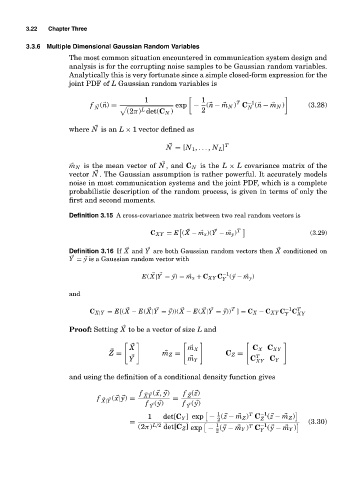
joint PDF of L Gaussian random variables is

1 1 T −1
N
f N ( n) = exp − ( n − m N ) C ( n − m N ) (3.28)
L
(2π) det(C N ) 2
where N is an L × 1 vector defined as

N = [N 1 , ... , N L ] T

m N is the mean vector of N , and C N is the L × L covariance matrix of the

vector N . The Gaussian assumption is rather powerful. It accurately models

noise in most communication systems and the joint PDF, which is a complete
probabilistic description of the random process, is given in terms of only the
first and second moments.

Definition 3.15 A cross-covariance matrix between two real random vectors is

T
C XY = E ( X − m x )( Y − m y ) (3.29)
Definition 3.16 If X and Y are both Gaussian random vectors then X conditioned on
Y = y is a Gaussian random vector with
−1
y
y
E( X| Y = ) = m x + C XY C ( − m y )
Y
and
T
C X|Y = E[( X − E( X| Y = y))( X − E( X| Y = y)) ] = C X − C XY C −1 C T XY
Y
Proof: Setting X to be a vector of size L and

X m X C X C XY

Z = m Z = C Z = T
Y m Y C XY C Y
and using the definition of a conditional density function gives

y
z
x
( , ) ( )
f X Y f Z
y
x
f X| Y ( | ) = =
y
y
( ) ( )
f Y f Y
−1
T
1

1 det[C Y ] exp − ( z − m Z ) C ( z − m Z )
Z
2
= L/2 1 −1 (3.30)
(2π) det[C Z ] exp − ( y − m Y ) C ( y − m Y )
T
2 Y