Page 106 - Fundamentals of Communications Systems

3.20 Chapter Three

Step 2:
y y
2
2
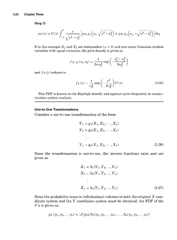
p Y (y) = U (y) p X 1 X 2 x 1 , y − x 1 2 + p X 1 X 2 x 1 , − y − x 2 1 dx 1
2
−y y − x 2
1
If in this example X 1 and X 2 are independent (ρ = 0) and zero mean Gaussian random
variables with equal variances, the joint density is given as
2
1 x + x 2 2
1
(x 1 , x 2 ) = exp −
f X 1 X 2 2 2
2πσ 2σ
X X
and f Y (y) reduces to
2
y y
f Y (y) = 2 exp − 2 U (y) (3.25)
σ 2σ
X X
This PDF is known as the Rayleigh density and appears quite frequently in commu-
nication system analysis.

One-to-One Transformations
Consider a one-to-one transformation of the form

Y 1 = g 1 (X 1 , X 2 , ··· , X n )

Y 2 = g 2 (X 1 , X 2 , ··· , X n )
.
.
.
Y n = g n (X 1 , X 2 , ··· , X n ) (3.26)

Since the transformation is one-to-one, the inverse functions exist and are
given as

X 1 = h 1 (Y 1 , Y 2 , ..., Y n )
X 2 = h 2 (Y 1 , Y 2 , ..., Y n )
.
.
.
X n = h n (Y 1 , Y 2 , ..., Y n ) (3.27)

Since the probability mass in infinitesimal volumes in both the original X coor-
dinate system and the Y coordinate system must be identical, the PDF of the
Y ’s is given as

p Y (y 1 , y 2 , ... y n ) =|J |p X (h 1 (y 1 , y 2 , ... y n ), ... , h n (y 1 , y 2 , ... y n ))