Page 305 - Fundamentals of Gas Shale Reservoirs

FLOW RATE DECLINE ANALYSIS 285

Oil production rate (BOPD) 100

–1
= 6%, EUR = 421 MBBLS
6-month history match: D = 32 mon , b = 2.0, d
min
i
–1
= 6%, EUR = 382 MBBLS
= 36 mon , b = 1.9, d
12-month history match: D i
min
–1
24-month history match: D = 36 mon , b = 1.1,
i
10 d min = 6%, EUR = 317 MBBLS
03 04 05 06 07 08
Years
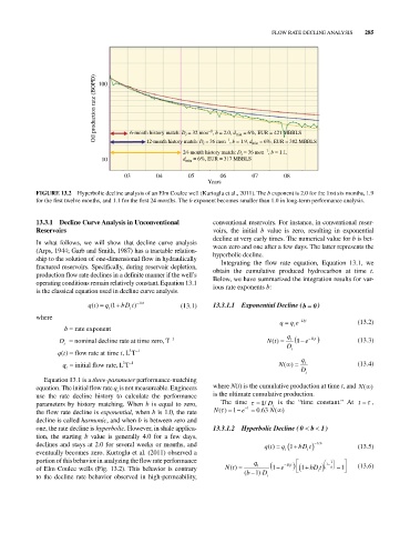
FIgURE 13.2 Hyperbolic decline analysis of an Elm Coulee well (Kurtoglu et al., 2011). The b exponent is 2.0 for the first six months, 1.9
for the first twelve months, and 1.1 for the first 24 months. The b exponent becomes smaller than 1.0 in long‐term performance analysis.
13.3.1 Decline Curve Analysis in Unconventional conventional reservoirs. For instance, in conventional reser-
Reservoirs voirs, the initial b value is zero, resulting in exponential
decline at very early times. The numerical value for b is bet-
In what follows, we will show that decline curve analysis ween zero and one after a few days. The latter represents the
(Arps, 1944; Garb and Smith, 1987) has a tractable relation- hyperbolic decline.
ship to the solution of one‐dimensional flow in hydraulically Integrating the flow rate equation, Equation 13.1, we
fractured reservoirs. Specifically, during reservoir depletion, obtain the cumulative produced hydrocarbon at time t.
production flow rate declines in a definite manner if the well’s Below, we have summarized the integration results for var-
operating conditions remain relatively constant. Equation 13.1 ious rate exponents b:
is the classical equation used in decline curve analysis.

qt() q (1 bDt) b / 1 (13.1) 13.3.1.1 Exponential Decline ( b 0 )
i i
where q q e Dt i (13.2)
b rate exponent i
q
D nominal declinerateat time zeroT 1 Nt() i 1 e Dt i (13.3)
,
i D
3
qt() flow rate at time t, LT 1 i
q
3
q initialflowrateL T 1 N() i (13.4)
,
i D
i
Equation 13.1 is a three‐parameter performance‐matching
equation. The initial flow rate q is not measureable. Engineers where N(t) is the cumulative production at time t, and ()N
i
use the rate decline history to calculate the performance is the ultimate cumulative production.
parameters by history matching. When b is equal to zero, The time 1 1/ D is the “time constant.” At t ,
i
the flow rate decline is exponential, when b is 1.0, the rate N() 1 e . 0 63 N( )
decline is called harmonic, and when b is between zero and
one, the rate decline is hyperbolic. However, in shale applica- 13.3.1.2 Hyperbolic Decline ( 0 b 1 )
tion, the starting b value is generally 4.0 for a few days,
declines and stays at 2.0 for several weeks or months, and qt() q 1 bDt b / 1 (13.5)
eventually becomes zero. Kurtoglu et al. (2011) observed a i i
portion of this behavior in analyzing the flow rate performance q 1 1
of Elm Coulee wells (Fig. 13.2). This behavior is contrary Nt() b ( i ) 1 D 1 e Dt i 1 bDt b 1 (13.6)
i
to the decline rate behavior observed in high‐permeability, i