Page 308 - Fundamentals of Gas Shale Reservoirs

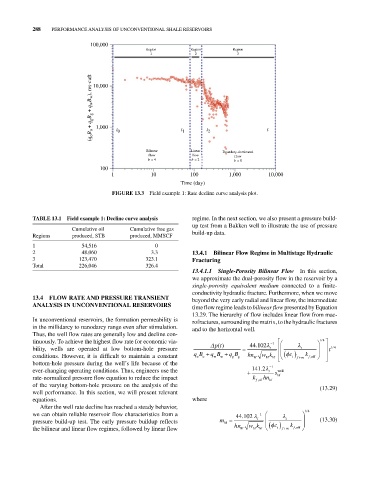
288 PERFORMANCE ANALYSIS OF UNCONVENTIONAL SHALE RESERVOIRS

100,000
Region Region Region
1 2 3

(q o B o + q g B g + q w B w ), res-cuft 10,000 t t t

1,000
t 0

Bilinear 1 Linear 2 Boundary-dominated
flow flow flow
b = 4 b = 2 b = 0
100
1 10 100 1,000 10,000
Time (day)
FIgURE 13.3 Field example 1: Rate decline curve analysis plot.

TABLE 13.1 Field example 1: Decline curve analysis regime. In the next section, we also present a pressure build‐
up test from a Bakken well to illustrate the use of pressure
Cumulative oil Cumulative free gas build‐up data.
Regions produced, STB produced, MMSCF
1 54,516 0
2 48,060 3.3 13.4.1 Bilinear Flow Regime in Multistage Hydraulic
3 123,470 323.1 Fracturing
Total 226,046 326.4
13.4.1.1 Single-Porosity Bilinear Flow In this section,
we approximate the dual‐porosity flow in the reservoir by a
single‐porosity equivalent medium connected to a finite‐
conductivity hydraulic fracture. Furthermore, when we move
13.4 FLOW RATE AND PRESSURE TRANSIENT beyond the very early radial and linear flow, the intermediate
ANALYSIS IN UNCONVENTIONAL RESERVOIRS time flow regime leads to bilinear flow presented by Equation
13.29. The hierarchy of flow includes linear flow from mac-
In unconventional reservoirs, the formation permeability is rofractures, surrounding the matrix, to the hydraulic fractures
in the millidarcy to nanodarcy range even after stimulation. and to the horizontal well.
Thus, the well flow rates are generally low and decline con-
tinuously. To achieve the highest flow rate for economic via- pt() 44 .102 1 14 /
bility, wells are operated at low bottom‐hole pressure t t t 14 /
conditions. However, it is difficult to maintain a constant qB o qB w qB g hn hf wk c t fm k f ,eff
w
o
g
hf hf
bottom‐hole pressure during the well’s life because of the 1
.
ever‐changing operating conditions. Thus, engineers use the 141 2 t s well
rate‐normalized pressure flow equation to reduce the impact k , f eff hn hf hf
of the varying bottom‐hole pressure on the analysis of the (13.29)
well performance. In this section, we will present relevant
equations. where
After the well rate decline has reached a steady behavior,
we can obtain reliable reservoir flow characteristics from a 44 102 1 14 /
.
pressure build‐up test. The early pressure buildup reflects m bl t c t k (13.30)
,
the bilinear and linear flow regimes, followed by linear flow hn hf wk t fm f eff
hf hf