Page 147 - Fundamentals of Magnetic Thermonuclear Reactor Design

Superconducting Magnet Systems Chapter | 5 129

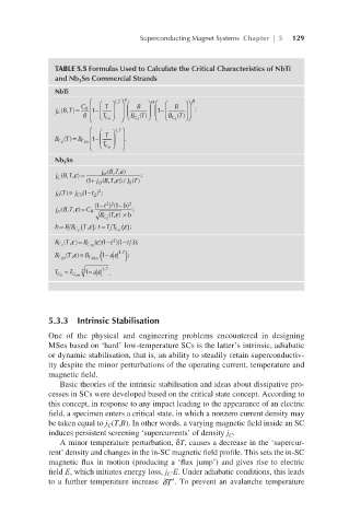
TABLE 5.5 Formulas Used to Calculate the Critical Characteristics of NbTi
and Nb 3 Sn Commercial Strands

NbTi
   1.7  γ      β
α
jB T) = C 0  1 −  T       B  1 −  B  ; jCB,T=C 0 B1−TTC 0 1.7γBBC 2 Tα1−-
(,
 

C
T
B    B ()    B ()  BBC 2 Tβ
T
  T C 0  C 2 C 2
   1.7 
B () = B C 20  1 −  T    . BC 2 T=BC201−TTC 0 1.7
T
C 2   
  T C 0 
Nb 3 Sn
ε
jB T,)
(,
ε =
cl
jB T,) ;
(,
C
(1 + jB T(, ε ,))/ 0 jCB,T,ε=jclB,T,ε1+jclB,T,ε/j 0 T
J T()
cl
2
jT() = j (1 −t ) ; j 0 T=jC 0 1−t 2
2
C0
2
0
22
(1 −t )(1 − b) 2
jB T,) ;
(,
ε = C 0
cl
B (, ε × b) 22 2
T
jclB,T,ε=C 0 1−t 1−b BC 2 T,ε×b
C 2
ε
/
C
= (T, t ε () ; b=B/BC 2 T,ε
=
T
t
bB B C 2 ε) ; = TT C 0 T 0
2
T
)
B (, ε = B C 20 ε ( )(1 −t )(1 −t 3); BC 2 T,ε=BC20ε1−t 1−t/3
2
C 2
T (, ) ( 1 − a ε 1.7 ) ;
m
B C 20 ε = B C 20
BC20T,ε=BC20m1−aε1.7
3 ε 1.7
T C 0 = T C m0 1 − a . TC 0 =TC0m1−aε1.73
5.3.3 Intrinsic Stabilisation
One of the physical and engineering problems encountered in designing
MSes based on ‘hard’ low-temperature SCs is the latter’s intrinsic, adiabatic
or dynamic stabilisation, that is, an ability to steadily retain superconductiv-
ity despite the minor perturbations of the operating current, temperature and
magnetic field.
Basic theories of the intrinsic stabilisation and ideas about dissipative pro-
cesses in SCs were developed based on the critical state concept. According to
this concept, in response to any impact leading to the appearance of an electric
field, a specimen enters a critical state, in which a nonzero current density may
be taken equal to j (T,B). In other words, a varying magnetic field inside an SC
C
induces persistent screening ‘supercurrents’ of density j .
C
A minor temperature perturbation, δT, causes a decrease in the ‘supercur-
rent’ density and changes in the in-SC magnetic field profile. This sets the in-SC
magnetic flux in motion (producing a ‘flux jump’) and gives rise to electric
field Е, which initiates energy loss, j ·Е. Under adiabatic conditions, this leads
C
to a further temperature increase Tδ ′. To prevent an avalanche temperature δT′