Page 106 - Fundamentals of Ocean Renewable Energy Generating Electricity From The Sea

Offshore Wind Chapter | 4 99

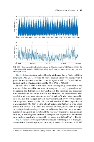
FIG. 4.14 Time series of hourly wind speed data at 100 m hub height at WIS Station 6309 for the
period 1980–2014, including 306,815 data points. The bottom plot shows a magnified view for a
sample year, 2014.
Fig. 4.14 shows the time series of hourly wind speed data at Station 6309 for
the period 1980–2014, covering 35 years. Because a leap year occurs every 4
years, the average number of data points for a year is 365.25 × 24 = 8766, and
the total number of data points would be 35 × 8766 = 306,810. 2
In order to fit a PDF to the wind speed, the frequency distribution of the
wind speed data should be evaluated. A histogram is a good graphical method
to represent the distribution of the wind speed. The minimum and maximum
wind speeds in the dataset are 0 and 36 m/s. Therefore, we can divide the wind
speed data into a series of intervals (or bins) from 0 to 36 m/s. Let us choose bin
sizes of 1 m/s. For example, the 12th bin will contain all recorded wind speeds
that are greater than or equal to 11.5 m/s and less than 12.5 m/s (regardless of
when recorded). The 13th bin includes all data points that have a wind speed
greater than or equal to 12.5 m/s and less than 13.5 m/s, and so forth. If we put
every single hourly wind speed observation/hindcast into a bin, we can sum the
number of data points in each bin. If the frequency (number of data points in
each bin) is plotted against the bins, a histogram will be produced. All of these
steps can be conveniently performed by computer (e.g. in MATLAB or Excel).
Fig. 4.15 shows the histogram of the wind data. In the top panel of this figure,
the number of cases (frequency of each bin) is shown. For instance, in 29,985

2. The actual number of data points is slightly different (306,815) in the downloaded dataset.