Page 199 - Fundamentals of Probability and Statistics for Engineers

182 Fundamentals of Probability and Statistics for Engineers

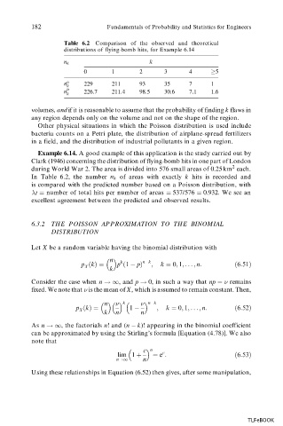
Table 6.2 Comparison of the observed and theoretical
distributions of flying-bomb hits, for Example 6.14
k
n k
0 1 2 3 4 5

n o 229 211 93 35 7 1
k
n p 226.7 211.4 98.5 30.6 7.1 1.6
k
volumes, and if it is reasonable to assume that the probability of finding k flaws in
any region depends only on the volume and not on the shape of the region.
Other physical situations in which the Poisson distribution is used include
bacteria counts on a Petri plate, the distribution of airplane-spread fertilizers
in a field, and the distribution of industrial pollutants in a given region.

Example 6.14. A good example of this application is the study carried out by
Clark (1946) concerning the distribution of flying-bomb hits in one part of London
2
during World War 2. The area is divided into 576 small areas of 0.25 km each.
In Table 6.2, the number n k of areas with exactly k hits is recorded and
is compared with the predicted number based on a Poisson distribution, with
t ˆ number of total hits per number of areas ˆ 537/576 ˆ 0.932. We see an
excellent agreement between the predicted and observed results.

6.3.2 THE POISSON APPROXIMATION TO THE BINOMIAL
DISTRIBUTION

Let X be a random variable having the binomial distribution with
n k n k

p k†ˆ p 1 p† ; k ˆ 0; 1; ... ; n: 6:51†
X
k
Consider the case when n !1,and p ! 0, in such a way that np ˆ remains

fixed. We note that is the mean of X, which is assumed to remain constant. Then,
n k n k

p k†ˆ 1 ; k ˆ 0; 1; ... ; n: 6:52†
X
k n n
As n !1 , the factorials n! and (n k)! appearing in the binomial coefficient
can be approximated by using the Stirling’s formula [Equation (4.78)]. We also
note that
c n

c
lim 1 ‡ ˆ e : 6:53†
n!1 n
Using these relationships in Equation (6.52) then gives, after some manipulation,

TLFeBOOK