Page 195 - Fundamentals of Probability and Statistics for Engineers

178 Fundamentals of Probability and Statistics for Engineers

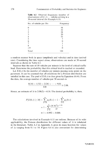
Table 6.1 Observed frequencies (number of
observations) of 0, 1, 2, . . . vehicles arriving in a
30-second interval (for Example 6.11)

No. of vehicles per 30 s Frequency
0 18
1 32
2 28
3 20
4 13
5 7
6 0
7 1
8 1
9 0
Total 120

a random manner both in space (amplitude and velocity) and in time (arrival
rate). Considering the time aspect alone, observations are made at 30-second
intervals as shown in Table 6.1.
Suppose that the rate of 10 vehicles per minute is the level of critical traffic
load. Determine the probability that this critical level is reached or exceeded.
Let X (0, t) be the number of vehicles per minute passing some point on the
pavement. It can be assumed that all conditions for a Poisson distribution are
satisfied in this case. The pmf of X (0, t) is thus given by Equation (6.44). From
the data, the average number of vehicles per 30 seconds is

0 18†‡ 1 32†‡ 2 28† ‡ ‡ 9 0†
 2:08:
120
Hence, an estimate of t is 2.08(2) ˆ 4:16. The desired probability is, then,

1 9
X X
P‰X 0; t† 10Šˆ p 0; t†ˆ 1 p 0; t†
k k
kˆ10 kˆ0
9 k 4:16
X 4:16† e
ˆ 1
k!
kˆ0
 1 0:992 ˆ 0:008:
The calculations involved in Example 6.11 are tedious. Because of its wide
applicability, the Poisson distribution for different values of t is tabulated
in the literature. Table A.2 in Appendix A gives its mass function for values
of t ranging from 0.1 to 10. Figure 6.4 is also convenient for determining

TLFeBOOK