Page 192 - Fundamentals of Probability and Statistics for Engineers

Some Important Discrete Distributions 175

No arrival No arrival

0 t t + t ∆
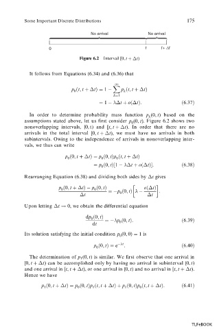
Figure 6.2 Interval [0, t ‡ t)

It follows from Equations (6.34) and (6.36) that
1
X
p t; t ‡ t†ˆ 1 p t; t ‡ t†
0 k
kˆ1
ˆ 1 t ‡ o t†: 6:37†

In order to determine probability mass function p (0, t) based on the
k
assumptions stated above, let us first consider p (0, t). Figure 6.2 shows two
0
nonoverlapping intervals, [0, t) and [t, t ‡ t). In order that there are no
arrivals in the total interval [0, t ‡ t), we must have no arrivals in both
subintervals. Owing to the independence of arrivals in nonoverlapping inter-
vals, we thus can write

p 0; t ‡ t†ˆ p 0; t†p t; t ‡ t†
0 0 0
ˆ p 0; t†‰1 t ‡ o t†Š: 6:38†
0
Rearranging Equation (6.38) and dividing both sides by t gives

p 0; t ‡ t† p 0; t† ˆ p 0; t† o t† :

0
0
t 0 t
Upon letting t ! 0, we obtain the differential equation
dp 0; t†
0 ˆ p 0; t†: 6:39†
dt 0
Its solution satisfying the initial condition p (0, 0) ˆ 1 is
0
p 0; t†ˆ e t : 6:40†
0
The determination of p 1 (0, t) is similar. We first observe that one arrival in
[0, t ‡ t) can be accomplished only by having no arrival in subinterval [0, t)
and one arrival in [t, t ‡ t), or one arrival in [0, t) and no arrival in [t, t ‡ t).
Hence we have

p 0; t ‡ t†ˆ p 0; t†p t; t ‡ t†‡ p 0; t†p t; t ‡ t†: 6:41†
1 0 1 1 0

TLFeBOOK