Page 210 - Fundamentals of Probability and Statistics for Engineers

Some Important Continuous Distributions 193

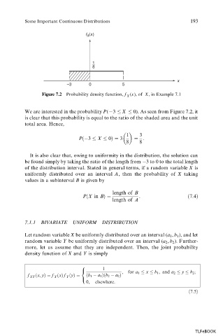
f (x)
X

1
—
8
x
–3 0 5

Figure 7.2 Probability density function, f (x), of X, in Example 7.1

X
We are interested in the probability P( 3 X 0). As seen from Figure 7.2, it

is clear that this probability is equal to the ratio of the shaded area and the unit
total area. Hence,
1 3

P 3 X 0†ˆ 3 ˆ :
8 8
It is also clear that, owing to uniformity in the distribution, the solution can
be found simply by taking the ratio of the length from 3 to 0 to the total length
of the distribution interval. Stated in general terms, if a random variable X is
uniformly distributed over an interval A, then the probability of X taking
values in a subinterval B is given by

length of B
P X in B†ˆ : 7:4†
length of A

7.1.1 BIVARIATE UNIFORM DISTRIBUTION

Let random variable X be uniformly distributed over an interval (a 1 , b 1 ), and let
random variable Y be uniformly distributed over an interval (a 2 , b 2 ). Further-
more, let us assume that they are independent. Then, the joint probability
density function of X and Y is simply

8
1
; for a 1 x b 1 ; and a 2 y b 2 ;
<
f XY x; y†ˆ f x† f y†ˆ b 1 a 1 † b 2 a 2 †
X
Y
:
0; elsewhere:
7:5†

TLFeBOOK