Page 43 - Fundamentals of Probability and Statistics for Engineers

26 Fundamentals of Probability and Statistics for Engineers

0.4 0.95
A 0.05 B

0.1

0.6 0.9
A B

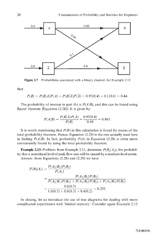
Figure 2.7 Probabilities associated with a binary channel, for Example 2.12

that

P B†ˆ P BjA†P A†‡ P BjA†P A†ˆ 0:95 0:4†‡ 0:1 0:6†ˆ 0:44:

The probability of interest in part (b) is P AjB), and this can be found using
Bayes’ theorem [Equation (2.28)]. It is given by:

P BjA†P A† 0:95 0:4†
P AjB†ˆ ˆ ˆ 0:863:
P B† 0:44

It is worth mentioning that P(B) in this calculation is found by means of the
total probability theorem. Hence, Equation (2.29) is the one actually used here
in finding P AjB). In fact, probability P(A) in Equation (2.28) is often more
conveniently found by using the total probability theorem.
Example 2.13. Problem: from Example 2.11, determine P B 2 jA 2 ), the probabil-
ity that a noncritical level of peak flow rate will be caused by a medium-level storm.
Answer: from Equations (2.28) and (2.29) we have

P A 2 jB 2 †P B 2 †
P B 2 jA 2 †ˆ
P A 2 †
P A 2 jB 2 †P B 2 †
ˆ
P A 2 jB 1 †P B 1 †‡ P A 2 jB 2 †P B 2 †‡ P A 2 jB 3 †P B 3 †
0:8 0:3†
ˆ ˆ 0:293:
1:0 0:5†‡ 0:8 0:3†‡ 0:4 0:2†

In closing, let us introduce the use of tree diagrams for dealing with more
complicated experiments with ‘limited memory’. Consider again Example 2.12

TLFeBOOK