Page 60 - Fundamentals of Probability and Statistics for Engineers

Random Variables and Probability Distributions 43

One can also give PDF and pmf a useful physical interpretation. In terms of
the distribution of one unit of mass over the real line 1 < x < 1, the PDF of
a random variable at x, F X 9x), can be interpreted as the total mass associated
x
with point x and all points lying to the left of . The pmf, in contrast, shows
the distribution of this unit of mass over the real line; it is distributed at discrete
with the amount of mass equal to p 9x i )at x i , i ˆ 1, 2, ....
points x i
X
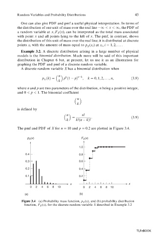
Example 3.2. A discrete distribution arising in a large number of physical
models is the binomial distribution. Much more will be said of this important
distribution in Chapter 6 but, at present, let us use it as an illustration for
graphing the PDF and pmf of a discrete random variable.
A discrete random variable X has a binomial distribution when

n n k

k
p k†ˆ p 1 p† ; k ˆ 0; 1; 2; ... ; n; 3:8†
X
k
n
where and p are two parameters of the distribution, n being a positive integer,
and 0 < p < 1. The binomial coefficient
n

k
is defined by
n n!

ˆ : 3:9†
k k! n k†!
0 2 are plotted in Figure 3.4.
The pmf and PDF of X for n ˆ 10 and p ˆ :

p X (x) F X (x)
1.0

0.4 0.8
0.3 0.6

0.2 0.4
0.1 0.2

x x
0 2 4 6 8 10 0 2 4 6 8 10

(a) (b)
( ), and (b) probability distribution
Figure 3.4 (a) Probability mass function, p x
X
function, F X x described in Example 3.2
( ), for the discrete random variable X

TLFeBOOK