Page 64 - Fundamentals of Probability and Statistics for Engineers

Random Variables and Probability Distributions 47

a case in which random variable X is continuously distributed over the real line
except at X ˆ 0, where P(X ˆ 0) is a positive quantity. This situation may arise
when, for example, random variable X represents the waiting time of a customer
at a ticket counter. Let X be the time interval from time of arrival at the ticket
counter to the time being served. It is reasonable to expect that X will assume
values over the interval X 0. At X ˆ 0, however, there is a finite probability of
not having to wait at all, giving rise to the situation depicted in Figure 3.7.
Strictly speaking, neither a pmf nor a pdf exists for a random variable of the
mixed type. We can, however, still use them separately for different portions of
the distribution, for computational purposes. Let f (x) be the pdf for the
X
continuous portion of the distribution. It can be used for calculating probabil-
ities in the positive range of x values for this example. We observe that the total
area under the pdf curve is no longer 1 but is equal to 1 P(X ˆ 0).
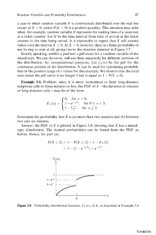
Example 3.4. Problem: since it is more economical to limit long-distance
telephone calls to three minutes or less, the PDF of X – the duration in minutes
of long-distance calls – may be of the form

0; for x < 0;
8
<
F X x†ˆ 1 e x=3 ; for 0 x < 3;
1 ; for x 3:
: e x=3
2
Determine the probability that X is (a) more than two minutes and (b) between
two and six minutes.
Answer: the PDF of X is plotted in Figure 3.8, showing that X has a mixed-
type distribution. The desired probabilities can be found from the PDF as
before. Hence, for part (a),
P X > 2†ˆ 1 P X 2†ˆ 1 F X 2†

ˆ 1 1 e 2=3 †ˆ e 2=3 :

F (x)
X

1
1– e ½
–
–1
1– e
x
3

Figure 3.8 Probability distribution function, F X (x), of X, as described in Example 3.4

TLFeBOOK