Page 98 - Fundamentals of Probability and Statistics for Engineers

Expectations and Moments 81

f (x)
X

1 σ

σ > σ 2
2
x
,and
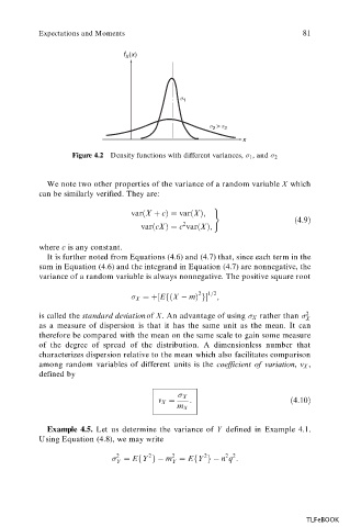
Figure 4.2 Density functions with different variances, 1 2

We note two other properties of the variance of a random variable X which
can be similarly verified. They are:

)
var X ‡ c†ˆ var X†;
4:9†
2
var cX†ˆ c var X†;
where c is any constant.
It is further noted from Equations (4.6) and (4.7) that, since each term in the
sum in Equation (4.6) and the integrand in Equation (4.7) are nonnegative, the
variance of a random variable is always nonnegative. The positive square root

2 1=2
X ˆ‡‰Ef X m† gŠ ;
is called the standard deviation of X. An advantage of using X rather than 2 X
as a measure of dispersion is that it has the same unit as the mean. It can
therefore be compared with the mean on the same scale to gain some measure
of the degree of spread of the distribution. A dimensionless number that
characterizes dispersion relative to the mean which also facilitates comparison
among random variables of different units is the coefficient of variation, v X ,
defined by

X
v X ˆ : 4:10†
m X

Example 4.5. Let us determine the variance of Y defined in Example 4.1.

Using Equation (4.8), we may write
2 2
2
2
2
2
ˆ EfY g m ˆ EfY g n q :
Y Y
TLFeBOOK