Page 127 - Fundamentals of Radar Signal Processing

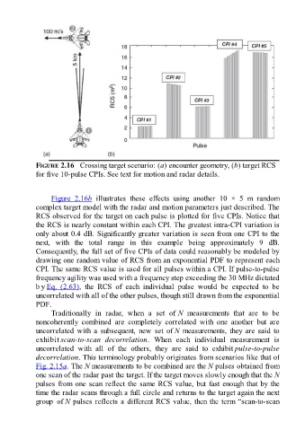
FIGURE 2.16 Crossing target scenario: (a) encounter geometry, (b) target RCS
for five 10-pulse CPIs. See text for motion and radar details.

Figure 2.16b illustrates these effects using another 10 × 5 m random
complex target model with the radar and motion parameters just described. The
RCS observed for the target on each pulse is plotted for five CPIs. Notice that
the RCS is nearly constant within each CPI. The greatest intra-CPI variation is
only about 0.4 dB. Significantly greater variation is seen from one CPI to the
next, with the total range in this example being approximately 9 dB.

Consequently, the full set of five CPIs of data could reasonably be modeled by
drawing one random value of RCS from an exponential PDF to represent each
CPI. The same RCS value is used for all pulses within a CPI. If pulse-to-pulse
frequency agility was used with a frequency step exceeding the 30 MHz dictated
b y Eq. (2.63), the RCS of each individual pulse would be expected to be
uncorrelated with all of the other pulses, though still drawn from the exponential

PDF.
Traditionally in radar, when a set of N measurements that are to be
noncoherently combined are completely correlated with one another but are
uncorrelated with a subsequent, new set of N measurements, they are said to
exhibit scan-to-scan decorrelation. When each individual measurement is
uncorrelated with all of the others, they are said to exhibit pulse-to-pulse
decorrelation. This terminology probably originates from scenarios like that of

Fig. 2.15a. The N measurements to be combined are the N pulses obtained from
one scan of the radar past the target. If the target moves slowly enough that the N
pulses from one scan reflect the same RCS value, but fast enough that by the
time the radar scans through a full circle and returns to the target again the next
group of N pulses reflects a different RCS value, then the term “scan-to-scan