Page 129 - Fundamentals of Radar Signal Processing

Examples include any of the PDFs in Table 2.3. For manmade targets, the

decorrelation model is usually taken as one of the extremes of either the fully
correlated or fully decorrelated models. Analysis carried out using these two
models produces bounding results for detection performance. In reality, the
noncoherently combined measurements will often be partially correlated. Partial
correlation models specified with a pulse-to-pulse correlation coefficient or an
autocorrelation function are sometimes given, though this is more common in

clutter modeling.

2.2.7 Swerling Models
An extensive body of radar detection theory has been built up using the four
Swerling models of target RCS fluctuation and noncoherent integration
(Swerling, 1960; Meyer and Mayer, 1973; Nathanson, 1991; Skolnik, 2001).
They are formed from the four combinations of two choices for the PDF and two
for the correlation properties. The two density functions used are the

exponential and the chi-square of degree 4 (see Table 2.3). The exponential
model describes the behavior of a complex target consisting of many scatterers,
none of which is dominant. The fourth-degree chi-square model targets having
many scatterers of similar strength with one dominant scatterer. Although the
Rice distribution is the exact PDF for this case, the chi-square is an
approximation based on matching the first two moments of the two PDFs (Meyer

and Mayer, 1973). These moments match when the RCS of the dominant
scatterer is times that of the sum of the RCS of the small scatterers,
so the fourth-degree chi-square model fits best for this case. More generally, a
2
chi-square of degree 2m = 1 + [a /(1 + 2a)] is a good approximation to a Rice
2
distribution with a ratio of a of the dominant scatterer to the sum of the small
scatterers. However, only the specific case of the fourth-degree chi-square is

considered a Swerling model.
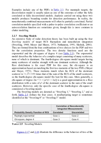
The Swerling models are denoted as “Swerling 1,” “Swerling 2,” and so
forth. Table 2.5 defines the four cases. A nonfluctuating target is sometimes
identified as the “Swerling 0” or “Swerling 5” model.

TABLE 2.5 Swerling Models

Figures 2.17 and 2.18 illustrate the difference in the behavior of two of the