Page 295 - Fundamentals of Radar Signal Processing

(4.125)

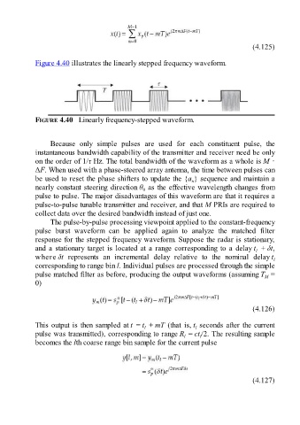
Figure 4.40 illustrates the linearly stepped frequency waveform.

FIGURE 4.40 Linearly frequency-stepped waveform.

Because only simple pulses are used for each constituent pulse, the
instantaneous bandwidth capability of the transmitter and receiver need be only
on the order of 1/τ Hz. The total bandwidth of the waveform as a whole is M ·
ΔF. When used with a phase-steered array antenna, the time between pulses can

be used to reset the phase shifters to update the {a } sequence and maintain a
n
nearly constant steering direction θ as the effective wavelength changes from
0
pulse to pulse. The major disadvantages of this waveform are that it requires a
pulse-to-pulse tunable transmitter and receiver, and that M PRIs are required to
collect data over the desired bandwidth instead of just one.
The pulse-by-pulse processing viewpoint applied to the constant-frequency
pulse burst waveform can be applied again to analyze the matched filter

response for the stepped frequency waveform. Suppose the radar is stationary,
and a stationary target is located at a range corresponding to a delay t + δt,
l
where δt represents an incremental delay relative to the nominal delay t l
corresponding to range bin l. Individual pulses are processed through the simple
pulse matched filter as before, producing the output waveforms (assuming T =
M
0)

(4.126)

This output is then sampled at t = t + mT (that is, t seconds after the current
l
l
pulse was transmitted), corresponding to range R = ct /2. The resulting sample
l
l
becomes the lth coarse range bin sample for the current pulse

(4.127)