Page 390 - Fundamentals of Radar Signal Processing

(5.99)

The algorithm finds the set of model coefficients {a } that optimally fits Ŷ(ω) to
p
Y(ω) for a given model order P. These coefficients are found by solving a set of
normal equations (Hayes, 1996) derived from the autocorrelation of the slow-

time data y[m]; the actual spectrum Y(ω) is not needed. The {ap} are then used
to compute an estimated spectrum according to Eq. (5.99), which can be
analyzed for target detection, pulse pair processing, or other functions.
Modeling the spectrum as shown in Eq. (5.99) is equivalent to modeling
the slow-time signal y[m] as the impulse response of an IIR filter with frequency
response . The inverse filter is an FIR filter with impulse
response coefficients h[m] = a and a = 1. If y[m] is passed through this filter
0
m
the output spectrum will be approximately constant provided that the actual
signal spectrum is accurately modeled by Eq. (5.99). It follows that if the {a }
p
2
are chosen such that |Ŷ(ω)| is a good model of the power spectrum of random
process data such as noise and clutter, then passing that data through the inverse
filter will produce a new random process with an approximately flat power

spectrum. Thus, the FIR filter designed from the model coefficients whitens the
signal, removing any correlated signal components such as clutter.
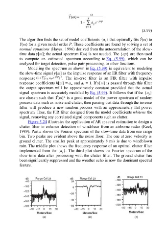
Figure 5.24 illustrates the application of AR spectral estimation to design a
clutter filter to enhance detection of windshear from an airborne radar (Keel,
1989). Part a shows the Fourier spectrum of the slow-time data from one range
bin. Two peaks are evident above the noise floor. The one at zero velocity is
ground clutter. The smaller peak at approximately 8 m/s is due to windblown

rain. The middle plot shows the frequency response of an optimal clutter filter
implemented from the {a }. The third plot shows the Fourier spectrum of the
p
slow-time data after processing with the clutter filter. The ground clutter has
been significantly suppressed and the weather echo is now the dominant spectral
feature.