Page 386 - Fundamentals of Radar Signal Processing

still large.

This problem can be avoided by ensuring that the sample set is dense
enough to guarantee that the three samples are all on the mainlobe. One way to
do this is to oversample in Doppler, i.e., choose K > M. Another is to window
the data. For most common windows, the expansion of the mainlobe that results
is sufficient to guarantee that the apparent peak samples and its two neighbors
fall on the same lobe, so that the basic assumption of a quadratic segment is

more valid. Figure 5.21b illustrates this effect by applying a Hamming window
to the same data used for Fig. 5.21a and again applying a 20-point DFT. Note
that the peak DTFT amplitude is now 10.34 due to the effect of the Hamming
window. Applying quadratic interpolation to this spectrum gives an estimated
spectral peak frequency and amplitude of 1336.6 Hz and 9.676, respectively,
errors of 6.4 percent in amplitude and 13.4 Hz in frequency. A hybrid technique
can be defined that combines attributes of the quadratic interpolation and the

more exact asinc interpolation. The parabolic method is used to identify the
frequency of the peak, and then Eq. (5.95) is used to estimate the amplitude.
This approach improves amplitude accuracy while avoiding the need to
compute Eq. (5.95) more than once.
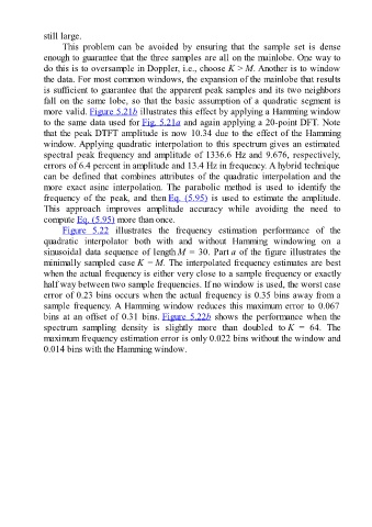
Figure 5.22 illustrates the frequency estimation performance of the
quadratic interpolator both with and without Hamming windowing on a

sinusoidal data sequence of length M = 30. Part a of the figure illustrates the
minimally sampled case K = M. The interpolated frequency estimates are best
when the actual frequency is either very close to a sample frequency or exactly
half way between two sample frequencies. If no window is used, the worst case
error of 0.23 bins occurs when the actual frequency is 0.35 bins away from a
sample frequency. A Hamming window reduces this maximum error to 0.067
bins at an offset of 0.31 bins. Figure 5.22b shows the performance when the

spectrum sampling density is slightly more than doubled to K = 64. The
maximum frequency estimation error is only 0.022 bins without the window and
0.014 bins with the Hamming window.