Page 505 - Fundamentals of Radar Signal Processing

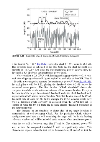
FIGURE 6.20 Example of cell-averaging CFAR threshold behavior.

–3
If the desired P = 10 , Eq. (6.121) gives the ideal T = 691, equal to 28.4 dB.
FA
This threshold level is indicated on the plot. Note that the ideal threshold is a
multiple of –ln(P ) = 6.91 times the true interference power; equivalently, the
FA
threshold is 8.4 dB above the interference power level.
Now consider a CA CFAR with leading and lagging windows of 10 cells

each after skipping a three-cell “guard region” to each side of the CUT. Thus N
15
= 20 cells are averaged to estimate the interference power. From Eq. (6.135),
the multiplier α will be 8.25, placing the threshold about 9.2 dB above the
estimated mean power. The line labeled “CFAR threshold” shows the
computed threshold as the reference window slides across the data. Except in
the vicinity of the target, the estimated threshold tracks the ideal threshold well,
staying within 2 dB across most of the data. Note that the data exceed the CFAR

threshold only at range bin 50. In this example the CFAR detector works very
well: a detection would correctly be declared when the CFAR test cell is
located at range bin 50, but there are no false alarms (threshold crossings) at
any other range bins.
The increase in the threshold to either side of the target location is
characteristic of cell-averaging CFAR. For the particular CFAR window

configuration used here the cell containing the target will be in the leading
reference window and will be included in the estimate of the interference power

when the test cell is between range bins 37 and 46. The estimated power

and, in turn, the computed threshold will be significantly raised. This
phenomenon repeats when the test cell is between bins 54 and 63 so that the